ВУЗ: Не указан
Категория: Не указан
Дисциплина: Не указана
Добавлен: 12.04.2021
Просмотров: 329
Скачиваний: 1

Icarus 139, 49–54 (1999)
Article ID icar.1999.6084, available online at http://www.idealibrary.com on
Catastrophic Resurfacing and Episodic Subduction on Venus
D. L. Turcotte, G. Morein, D. Roberts, and B. D. Malamud
Department of Geological Sciences, Cornell University, Ithaca, New York 14853-1504
E-mail: turcotte@geology.cornell.edu
Received March 3, 1998; revised September 4, 1998
There is clear evidence that a catastrophic resurfacing event oc-
curred on Venus in the relatively recent past. A primary data source
for this resurfacing event is the spatial distribution of impact craters.
In this paper, we apply the pair-correlation technique to the ob-
served crater distribution and find that the result is identical to
that for a random distribution. In order to test the sensitivity of
the technique, we also apply it to the spatial distribution of coronae
on Venus. For the coronae, we find substantial deviations from a
random distribution. One explanation for the catastrophic resur-
facing is the episodic subduction hypothesis. We model episodic
subduction using a thermal boundary-layer stability analysis. We
find that episodic subduction events with intervals of 500 to
700 Myr can transport only 15–25% of the radiogenic heat pro-
duced within the planet. We suggest that the remainder of the heat
must be lost to the surface during a period of vigorous tectonic ac-
tivity, following the subduction event but prior to the subsequent
stabilization of a global lithosphere.
c
°
1999 Academic Press
Key Words:
Venus; tectonics; cratering; heat flow; mantle convec-
tion.
INTRODUCTION
One of the most important results of the Magellan mission to
Venus was the information provided on the tectonic evolution of
the planet. Two major conclusions are now generally accepted:
(1) Venus does not have plate tectonics as we know it on
Earth. There is no evidence for a global pattern of accretional
plate margins and subduction zones.
(2) The age of the surface of Venus is nearly uniform and is
neither very old (heavily cratered) nor very young (very lightly
cratered).
Other observed features of the venusian surface also provide
important insights into the global tectonic evolution of the planet.
It is necessary to explain the regions of elevated topography and
the coronae. There does not appear to be any analogs to coronae
on Earth.
The essential question in understanding the tectonic evolution
of Venus is to understand how it loses heat. Based on our knowl-
edge of Earth, it is reasonable to conclude that this loss of heat
would be associated with the instability and subduction of the
lithosphere. However, without plate tectonics, how does subduc-
tion occur? Turcotte (1993, 1995) proposed that episodic global
subduction events occur on Venus. Parmentier and Hess (1992)
associate episodic subduction with a chemical instability of the
lithosphere. An alternative hypothesis is that Venus had active
plate tectonics like Earth during its early evolution, but that the
global lithosphere subsequently stabilized and Venus is now in
a transient state between plate tectonics (Earth) and lithospheric
conduction (Mars) (Arkani-Hamed and Toksoz 1984, Arkani-
Hamed et al. 1993, Arkani-Hamed 1994).
It is expected that Venus will have concentrations of the heat-
producing elements uranium, thorium, and potassium, similar
to the concentrations found in Earth. If the heat generated by
those elements is to be lost at the surface, then either the heat
must be conducted through a stable lithosphere or the lithosphere
must be subject to episodic subduction. The alternative is that
the temperature within the planet is increasing. In the long term,
such heating must lead to some kind of a catastrophic event.
On Earth, the internal radiogenic heating generates mantle
convection. Earth’s lithosphere is the cold thermal boundary
layer associated with this convection. The thermal instability of
the lithosphere leads to its subduction at ocean trenches and its
continuous replacement at ocean ridges. This is plate tecton-
ics. The cooling of Earth’s interior due to the subducted cold
lithosphere constitutes some 70% of the heat transfer out of the
mantle. The remainder can be attributed to delamination (partial
subduction) of the lithosphere and to hot mantle plumes that are
associated with the instability of a hot thermal boundary layer
at depth.
In this paper, we address two aspects of the tectonic evolution
of Venus: first, we consider whether the distribution of craters
on Venus is random, and second, we consider a simple param-
eterized convection model for episodic subduction. Cratering
statistics are the primary data base for establishing the age dis-
tribution of the venusian surface. Although it is well established
that a catastrophic resurfacing event occurred, the time progres-
sion of resurfacing has been open to considerable debate. We
apply the pair-correlation technique to the spatial distribution
of craters on Venus in order to quantify the randomness of the
distribution.
We also consider a simple parameterized model for episodic
convection on Venus. This model is based on boundary-layer
49
0019-1035/99 $30.00
Copyright c
°
1999 by Academic Press
All rights of reproduction in any form reserved.
50
TURCOTTE ET AL.
stability criteria for a thickening thermal lithosphere. The tem-
poral evolution of the mantle temperature and viscosity and the
thickness of the lithosphere are determined.
CRATERING STATISTICS
The hypothesis of a global resurfacing event on Venus is
largely based on the distribution of impact craters over the sur-
face of the planet. On both the Moon and Mars, ancient surfaces
are clearly differentiated from younger surfaces by large dif-
ferences in crater densities. The earliest results from Magellan
indicated that this was not the case for Venus. The density of
craters over the surface of Venus appeared to be essentially uni-
form and this led to the hypothesis of a global resurfacing event
(Schaber et al. 1992).
It is clearly desirable to quantify just how uniform the dis-
tribution of craters over the surface of Venus is. In order to do
this, Strom et al. (1994) carried out Monte-Carlo simulations
in which totally random distributions of craters were obtained.
The actual distribution of craters could not be visually distin-
guished from the random simulations. In this paper, we wish to
systematically quantify the randomness of the crater distribution
on Venus. A standard approach to this problem is to obtain pair-
correlation statistics (Kagan and Knopoff 1980, Turcotte 1997).
In this method, the distance from each crater to all other craters
is determined. We assume Venus to be a sphere so that the range
of distances between craters is from r
=
0 to r
=
π
a, where a is
the radius of the planet. The length r is measured along the sur-
face of the sphere. The probability distribution function, f (r
/
a),
for these distances is then obtained.
Before proceeding with Venus, we obtain the results we would
expect for a random distribution of points (craters) over the sur-
face of a sphere. In order to do this, we pick one point and con-
FIG. 1.
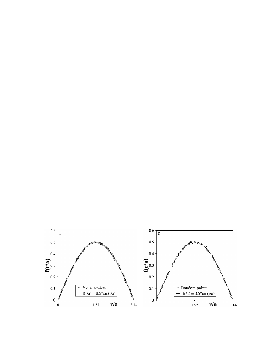
(a) Pair-correlation technique applied to 923 craters on Venus. The probability distribution function for distances between craters, f (r
/
a), is given
as a function of (r
/
a). (b) Pair-correlation technique applied to 923 points randomly distributed over a sphere. The probability distribution function for distances
between points, f (r
/
a), is given as a function of (r
/
a). In both cases, the data are compared with the analytical prediction for a random distribution given in (1).
For the Venus craters we find r
2
=
0
.
9996 and for the 923 random points we find r
2
=
0
.
9994.
sider the distribution of other points as a function of the distance
r from the point chosen. In the immediate vicinity of the chosen
point, the number of adjacent random points will increase in
proportion to r , the maximum number of random points will be
at r
/
a
=
π
/2, and the number of random points will approach
zero as r
/
a
→
π
. The increment of area at a distance r from
the chosen point is 2
π
a
2
sin
θ
d
θ
where d
θ
=
dr
/
a. Thus, the
expected probability distribution function for points randomly
distributed over the surface of Venus is
f (r
/
a)
=
0
.
5 sin(r
/
a)
.
(1)
The probability distribution function for the pair-correlation
statistics of random points on a sphere is a sine function.
We have obtained the pair-correlation statistics for 923 craters
on Venus using data from Herrick et al. (1997). Because of the
very large number of pair-correlation data points,
≈
10
6
, the data
are binned with bin width
1
r
/
a
=
0
.
05. The binned data cor-
responding to the probability distribution function f (r
/
a) are
given in Fig. 1a. We compare this to the analytical prediction
given in (1). As a measure of agreement we use the Pearson prod-
uct moment correlation coefficient, r , which is a dimensionless
index that ranges for
−
1.0 to 1.0 and reflects the extent of a linear
relationship between two data sets. For the data shown in Fig. 1a
we have r
2
=
0
.
9996. In order to further test the agreement of the
crater statistics with a random distribution we obtain the pair-
correlation statistics for 923 points randomly distributed over a
sphere, the resulting binned data are given in Fig. 1b. Again, we
compare the random simulation data with the analytical predic-
tion given in (1). In this case r
2
=
0
.
9994. The crater data are
essentially indistinguishable from the random data. In addition,
both the crater data and the random data coincide very closely
with the analytic relation given in (1). In fact the crater data with
CATASTROPHIC RESURFACING AND EPISODIC SUBDUCTION ON VENUS
51
r
2
=
0
.
9996 are slightly closer to the analytic relation (1) then
the random simulation with r
2
=
0
.
9994.
Although the results given in Fig. 1 indicate no significant
differences between the distribution of craters and a random
distribution, it is also of interest to determine how sensitive the
pair-correlation technique is to deviations. In order to provide
a comparative test we consider the pair-correlation statistics for
the distributions of coronae on Venus. Using nearest-neighbor
statistics, Squyres et al. (1993) concluded that the spatial distri-
bution of coronae on Venus is fractal rather than random. The
spatial distribution of hostspots on Earth is also fractal (Jurdy and
Stefanick 1990). Both the coronae on Venus and the hotspots on
Earth are clustered relative to a random distribution. Because of
this clustering, we would expect that the pair-correlation statis-
tics for the coronae would deviate significantly from random
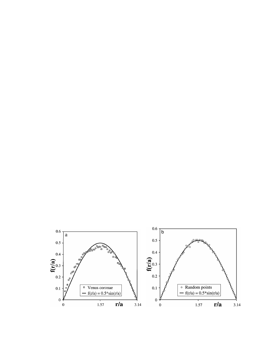
simulations. We have obtained the pair-correlation statistics for
335 coronae on Venus; the results for the binned probability
distribution function f (r
/
a) are given in Fig. 2a. Again, the
pair-correlation statistics are compared with the analytical pre-
diction given in (1). For the data shown in Fig. 2a we have
r
2
=
0
.
9690. This relatively low value quantifies the obvious
differences between the coronae data and the random prediction
(1). Once again, we make a direct comparison with a random
simulation. The pair-correlation statistics for 335 points ran-
domly distributed over sphere are given in Fig. 2b. Again the
data are compared with the analytical prediction given in (1),
in this case r
2
=
0
.
9971. This value is somewhat lower than the
r
2
=
0
.
9994 for the random simulation given in Fig. 1b, the in-
creased scatter in Fig. 2b can be attributed to the smaller number
of random points considered. However, the random simulation
is much closer to the analytical prediction than the coronae data.
There are several significant differences between the data
given in Figs. 1a and 2a. First, there is considerably more scat-
FIG. 2.
(a) Pair-correlation technique applied to 335 coronae on Venus. The probability distribution function for distances between craters, f (r
/
a), is given
as a function of (r
/
a). (b) Pair-correlation technique applied to 335 points randomly distributed over sphere. The probability distribution function for distances
between points, f (r
/
a), is given as a function of (r
/
a). In both cases the data are compared with the analytical prediction for a random distribution given in (1).
For the Venus Coronae we find r
2
=
0
.
9690 and for the 335 random points we find r
2
=
0
.
9971.
ter for the pair-correlation statistics of coronae than for craters.
This can be attributed to the smaller number of coronae con-
sidered. Even with this scatter, it is clear from Fig. 2 that there
are significant differences between the coronae data and the ran-
dom data. For small separations, (r
/
a)
<
1, the coronae data lie
systematically above the random data. For larger separations,
1
<
(r
/
a)
<
2
.
5, the coronae data lie systematically below the
random data.
When data are clustered, small separations of points are dom-
inant over large separations. Thus, the pair-correlation statistics
for coronae given in Fig. 2 are consistent with clustering rel-
ative to a random distribution. If there were significant varia-
tions in age over the surface of Venus then there would also
be significant variations in crater densities relative to a random
distribution. This is clustering. Thus, significant variations in
the age of the surface of Venus over significant areas would be
expected to give large values of f (r
/
a) for small r
/
a. There is
no evidence for this clustering in the pair-correlation statistics
for venutian craters given in Fig. 1. Thus, we conclude that the
pair-correlation data confirm the previous conclusion that the
spatial distribution of craters on Venus is indistinguishable from
a random distribution.
IMPLICATIONS OF CRATERING STATISTICS
There is conclusive evidence for a “catastrophic” resurfac-
ing event on Venus. There are no “heavily cratered” regions
on Venus. Thus, there is no evidence for “old” lithosphere on
Venus as there is on Earth in the continental cratons. Since there
must have been lithosphere on Venus at all times in the past,
the evidence is that this lithosphere was “destroyed” either by
subduction or by extensive internal deformation.

52
TURCOTTE ET AL.
Although we can say conclusively that the surface of Venus
has been resurfaced in the relatively recent past, say 500 Ma,
the temporal history of the resurfacing is open to question. Un-
certainties in the absolute cratering record for Venus lead to
uncertainties in the age of the surface. It is probably reasonable
to say that the resurfacing was centered at 500
±
200 Ma. Phys-
ically, the resurfacing must have spanned some length of time,
it certainly did not occur instantaneously.
A number of authors have examined the surface evidence for
the temporal distribution of volcanism on Venus (Bullock et al.
1993, Herrick 1994, Namiki and Solomon 1994, Price and Suppe
1994). Various estimates have been given for the age distribu-
tion of the Venus surface. Because the results are sensitive to
the assumed areal distribution of more recent volcanic flows, it
is very difficult to provide quantitative constraints on the age
history of the surface of Venus. We will present two hypothet-
ical end-member models for the surface age distribution: a fast
resurfacing model and a slow resurfacing model.
For the fast resurfacing model, we assume that the oldest
surface is 600 Ma. We further assume that 90% of the surface
was resurfaced in 10 Myr and 98% of the surface was resurfaced
in 50 Myr. For the slow resurfacing model, we again assume that
the oldest surface is 600 Ma. We assume that 70% of the surface
was resurfaced in 30 Myr, 90% in 100 Myr, and 98% in 300 Myr.
From a tectonic prospective, the principal differences between
the two end-member models is the role of continuing volcanic
and tectonic processes versus the creation of the new lithosphere
to replace old lithosphere.
EPISODIC SUBDUCTION MODEL
If it is accepted that episodic global subduction of the litho-
sphere on Venus is the primary mechanism for heat loss, it is
clearly desirable to quantify the mechanism. In order to do
this, we consider a parameterized boundary-layer model for
high Rayleigh number thermal convection. This model was pro-
posed by Howard (1966) for turbulent thermal convection. In
this model it is assumed that the upper thermal boundary layer
(the lithosphere) becomes unstable and sinks (subducts) when
the Rayleigh number based on the thickness of the lithosphere
Y
L
reaches a critical value Ra
cr
. We hypothesize that a global
subduction event occurs when
Ra
cr
=
ρ
m
g
α
[T
m
(t )
−
T
s
]Y
3
L
η
(t )
κ
,
(2)
where
ρ
m
=
4500 kg m
−
3
is the average mantle density, g
=
8
.
6 m s
−
2
is the surface gravity on Venus,
α
=
2
.
4
×
10
−
5
K
−
1
is
the thermal expansion coefficient, T
s
(t ) is the mean mantle tem-
perature, T
s
=
750 K is the surface temperature, and
κ
=
10
−
6
m
2
s
−
1
is the thermal diffusivity. The mantle viscosity
η
(t ) is
itself a strong function of the mantle temperature,
η
(t)
=
Ce
E a
RTm(t )
,
(3)
with constant C
=
1
.
414
×
10
4
Pa s, activation energy E
a
=
5
.
23
×
10
5
J mol
−
1
, and gas constant R
=
8
.
31 J mol
−
1
K
−
1
.
After a global subduction event there are two important effects
that increase the Rayleigh number. The first is the increase in the
thickness of the lithosphere Y
L
in time; the second is the decrease
in mantle viscosity
η
(t ) as the interior mantle temperature T
m
in-
creases. The Rayleigh number of the lithosphere increases until
it reaches the critical value, Ra
cr
, and another global subduction
event occurs.
We assume that Venus has the same rate of radiogenic heat
production per unit mass, H (t ), as Earth. We further assume
that the heat production within Venus can be approximated by
(Turcotte and Schubert 1982, p. 332)
H (t )
=
H
0
e
−
λ
(t
−
t
0
)
,
(4)
where H
0
=
6
.
18
×
10
−
12
W kg
−
1
is the present heat produc-
tion, t
0
is the age of Earth, t is time measured forward, and
λ
=
2
.
77
×
10
−
10
year
−
1
. We assume that between global sub-
duction events the radiogenic heat production heats the mantle
and write
C
dT
m
(t)
dt
=
H (t)
,
(5)
where C is the specific heat. The solution of (4) and (5) is
T
m
(t)
=
T
m
(t
s
)
+
H
0
e
λ
t
0
C
λ
¡
e
−
λ
t
s
−
e
−
λ
t
¢
,
(6)
where t
s
is the time of the last subduction event. The corre-
sponding thickness of the lithosphere is given by (Turcotte and
Schubert 1982, p. 164)
Y
L
(t)
=
2
.
32[
κ
(t
−
t
s
)]
1/2
.
(7)
Solutions of (3), (6), and (7) give the dependence on time of
the mantle temperature T
m
, mantle viscosity
η
(t ), and the litho-
spheric thickness Y
L
(t) between subduction events.
In order to complete the formulation of the problem we must
specify the heat loss from the mantle during a subduction event.
We assume that this is made up of two parts: The first part is
due to the subduction of cold lithosphere and the second part is
the loss of heat to the surface before a new global lithosphere
stabilizes. Under these assumptions, the change in the mantle
temperature due to a global subduction event,
1
T
m
, is given
by
1
T
m
=
(T
m
(t)
−
T
s
)
ρ
l
£
R
3
v
−
(R
v
−
Y
L
)
3
¤
1
.
16
√
πρ
m
(R
v
−
Y
L
)
3
−
1
T
,
(8)
where
ρ
l
is the density of the lithosphere, R
v
the radius of Venus,
and
1
T is the prescribed loss of temperature before a new litho-
sphere stabilizes.
CATASTROPHIC RESURFACING AND EPISODIC SUBDUCTION ON VENUS
53
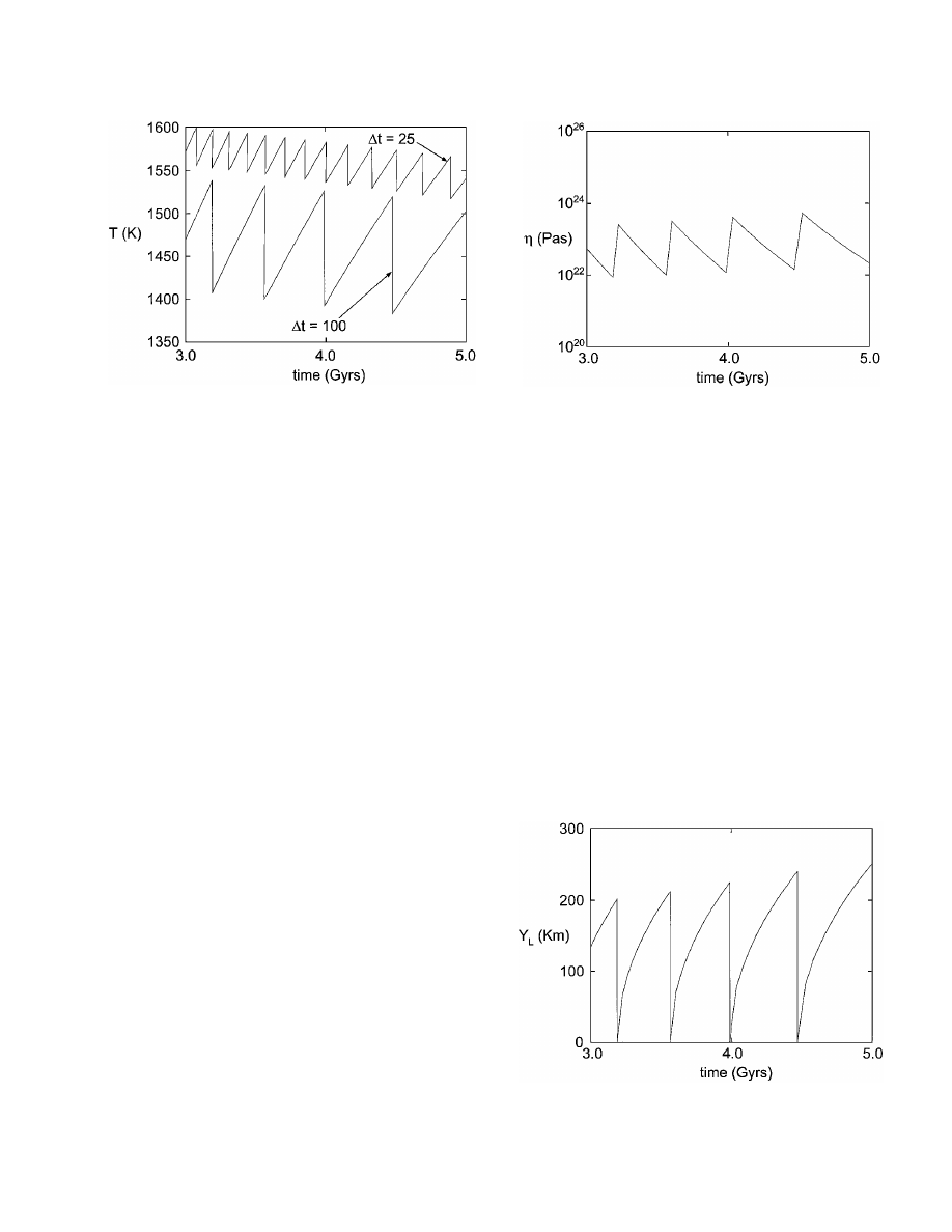
FIG. 3.
Values of the mantle temperature in Venus, T
m
, as a function of
time, t. Results are given for prescribed temperature losses
1
T
=
25 and 100 K.
In order to solve this problem an initial mantle temperature
for the planet is assumed, T
m
=
T
m0
at t
=
0. Equations (3), (6),
and (7) are solved numerically to give T
m
(t )
, η
(t ), and Y
L
(t);
these values are then substituted into the stability criteria (2)
until it is satisfied. When it is satisfied a global subduction event
is assumed to have occurred. The change in the mantle temper-
ature due to the subduction event is determined from (8) and
the process is repeated. After a few subduction events, the ther-
mal evolution of the mantle is insensitive to the initial mantle
temperature T
m0
.
A number of simulations have been carried out using the nu-
merical values given above and various values of the heat loss
parameter
1
T . Values of the mantle temperature in Venus, T
m
as a function of time t, are given in Fig. 3, with
1
T
=
25 and
100 K. With
1
T
=
25 K, global subduction events occur at in-
tervals of about 150 Myr. This is clearly not consistent with
our understanding of Venus. However, it is consistent with plate
tectonics on Earth. For Earth it is appropriate to take
1
T
=
0,
and our analysis would predict that subduction would occur at
intervals of about 125 Myr. This is close to the average age of
subducting lithosphere on Earth.
In order to get longer intervals between global subduction
events it is necessary to increase
1
T . With
1
T
=
100 K we find
the intervals to be about 500 Myr as shown in Fig. 3. Thus, ap-
proximately 75% of the heat loss from the interior of Venus must
occur after a global subduction event and prior to the establish-
ment of a new global lithosphere. The values of mantle viscosity
and lithosphere thickness in this simulation are given in Figs. 4
and 5. The mantle viscosity oscillates between values of about
10
22
and 10
24
Pa. This two orders of magnitude decrease in the
mantle viscosity during the mantle heating phase contributes
substantially to the instability of the lithosphere, leading to a
global subduction event. The lithosphere thickness increases to
a value Y
L
≈
250 km prior to subduction.
It should be emphasized that the parameterized boundary-
layer model is highly idealized. An alternative approach would
FIG. 4.
Values of the mantle viscosity,
η
, as a function of time t, with
1
T
=
100 K.
be to consider full numerical models of thermal convection.
Solomatov and Moresi (1996, 1997) have carried out numer-
ical calculations of thermal convection within Venus, including
both a strong temperature dependence and a nonlinear rheology.
Because of the strong temperature dependence, a stagnant lid
(rigid global lithosphere) is found under a wide range of param-
eter values. A basic question is whether the fluid approach can
reasonably model the subduction of a lithosphere with a strongly
temperature-dependent rheology. Since our primary purpose is
to model the subduction of a thickening thermal lithosphere,
the boundary-layer instability approach seems to be appropri-
ate. The fact that it successfully predicts the age of subducting
lithosphere on Earth is a verification of the approach. A prin-
cipal result of our analysis is that the subduction of a global
lithosphere on Venus at intervals of 500 Myr or more can only
transport a small fraction of the heat being generated within the
FIG. 5.
Values of the lithospheric thickness, Y
L
, as a function of time t ,
with
1
T
=
100 K.