Файл: Introduction to Python for Science 2013.pdf

Introduction to Python for Science, Release 0.9.23

4

3

2

1

0

1

2

3

4

5

x

0.0

0.2

0.4

0.6

0.8

1.0

1.2

P(x)

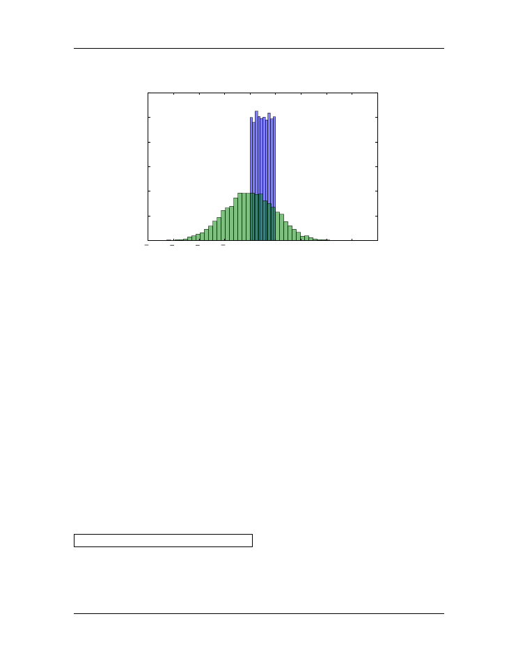
Figure 3.1: Histograms of random numbers.

3.5.3 Random distribution of integers

The function

randint(low, high, num)

produces a uniform random distribution

of

num

integers between

low

(inculsive) and

high

(exclsusive). For example, we can

simulate a dozen rolls a single die with the following statement

In [7]:

randint(

1

,

7

,

12

)

Out[7]:

array([

6

,

2

,

1

,

5

,

4

,

6

,

3

,

6

,

5

,

4

,

6

,

2

])

3.5.4 Loading random number functions

When working within the IPython shell, you can use the random number functions simply
by writing

rand(10)

,

randn(10)

, or,

randint(10)

, because the

np.random

library is loaded when IPython is launched. However, to use these functions in a script
or program, you need to load them from the

numpy.random

library, as discussed in

section on

Importing Modules

, and as illustrated in the above program for making the

histogram in the above figure.

Recap of random number generators

Random number generators

must

be

imported

from

the

numpy.random

library.

For

more

information,

see

http://docs.scipy.org/doc/numpy/reference/routines.random.html

50

Chapter 3. Strings, Lists, Arrays, and Dictionaries

Introduction to Python for Science, Release 0.9.23

rand(num)

generates an array of

num

random floats uniformly distributed

on the interval from 0 to 1.

randn(num)

generates an array of

num

random floats normally distributed

with a width of 1.

randint(low, high, num)

generates an array of

num

random inte-

gers between

low

(inclusive) and

high

exclusive.

3.5. Random numbers

51

Introduction to Python for Science, Release 0.9.23

3.6 Exercises

1. Create at array of 9 evenly spaced numbers going from 0 to 29 (inclusive) and give

it the variable name

r

. Find the square of each element of the array (as simply as

possible). Find twice the value of each element of the array in two different ways:
(

i

) using addition and (

ii

) using multiplication.

2. Create the following arrays:

(a) an array of 100 elements all equal to

e

, the base of the natural logarithm;

(b) an array in 1-degree increments of all the angles in degrees from 0 to 360

degrees;

(c) an array in 1-degree increments of all the angles in radians from 0 to 360

degrees;

(d) an array from 12 to 17, not including 17, in 0.2 increments;

(e) an array from 12 to 17, including 17, in 0.2 increments.

3. The position of a ball at time

t

dropped with zero initial velocity from a height

h

0

is given by

y

=

h

0

−

1
2

gt

2

where

g

= 9

.

8 m

/

s

2

. Suppose

h

0

= 10 m

. Find the sequence of times when the

ball passes each half meter assuming the ball is dropped at

t

= 0

. Hint: Create a

NumPy array for

y

that goes from 10 to 0 in increments of -0.5 using the

arange

function. Solving the above equation for

t

, show that

t

=

s

2(

h

0

−

y

)

g

.

Using this equation and the array you created, find the sequence of times when the
ball passes each half meter. Save your code as a Python script. It should yield the
following results for the

y

and

t

arrays:

In [2]:

y

Out[2]:

array([

10.

,

9.5

,

9.

,

8.5

,

8.

,

7.5

,

7.

,

6.5

,

6. , 5.5, 5. , 4.5, 4. , 3.5, 3. , 2.5,

2. , 1.5, 1. , 0.5])

In [3]:

t

Out[3]:

array([

0.

,

0.31943828

,

0.45175395

,

52

Chapter 3. Strings, Lists, Arrays, and Dictionaries

Introduction to Python for Science, Release 0.9.23

0.55328334, 0.63887656, 0.71428571,

0.7824608 , 0.84515425, 0.9035079 ,

0.95831485, 1.01015254, 1.05945693,

1.10656667, 1.15175111, 1.19522861,

1.23717915, 1.27775313, 1.31707778,

1.35526185, 1.39239919])

4. Recalling that the average velocity over an interval

∆

t

is defined as

¯

v

= ∆

y/

∆

t

,

find the average velocity for each time interval in the previous problem using
NumPy arrays. Keep in mind that the number of time intervals is one less than
the number of times. Hint: What are the arrays

y[1:20]

and

y[0:19]

? What

does the array

y[1:20]-y[0:19]

represent? (Try printing out the two arrays

from the IPython shell.) Using this last array and a similar one involving time,
find the array of average velocities. Bonus: Can you think of a more elegant way
of representing

y[1:20]-y[0:19]

that does not make explicit reference to the

number of elements in the

y

array—one that would work for any length array?

You should get the following answer for the array of velocities:

In [5]:

v

Out[5]:

array([

-

1.56524758

,

-

3.77884195

,

-

4.9246827

,

-5.84158351,

-6.63049517,

-7.3340579 ,

-7.97531375,

-8.56844457,

-9.12293148,

-9.64549022,

-10.14108641, -10.61351563,

-11.06575711, -11.50020061, -11.91879801,

-12.32316816, -12.71467146, -13.09446421,

-13.46353913])

3.6. Exercises

53

Introduction to Python for Science, Release 0.9.23

54

Chapter 3. Strings, Lists, Arrays, and Dictionaries