ВУЗ: Не указан
Категория: Не указан
Дисциплина: Не указана
Добавлен: 17.04.2021
Просмотров: 3756
Скачиваний: 3

CHAPTER
SEVEN
FUNCTIONS
As you develop more complex computer code, it becomes increasingly important to or-
ganize your code into modular blocks. One important means for doing so is
user-defined
Python functions. User-defined functions are a lot like built-in functions that we have
encountered in core Python as well as in NumPy and Matplotlib. The main difference is
that user-defined functions are written by you. The idea is to define functions to simplify
your code and to allow you to reuse the same code in different contexts.
The number of ways that functions are used in programming is so varied that we cannot
possibly enumerate all the possibilities. As our use of Python functions in scientific pro-
gram is somewhat specialized, we introduce only a few of the possible uses of Python
functions, ones that are the most common in scientific programming.
7.1 User-defined functions
The NumPy package contains a plethora of mathematical functions.
You can find
a listing of the mathematical functions available through NumPy on the web page
http://docs.scipy.org/doc/numpy/reference/routines.math.html
. While the list may seem
pretty exhaustive, you may nevertheless find that you need a function that is not available
in the NumPy Python library. In those cases, you will want to write your own function.
In studies of optics and signal processing one often runs into the sinc function, which is
defined as
sinc
x
≡
sin
x
x
.
Let’s write a Python function for the sinc function. Here is our first attempt:
115

Introduction to Python for Science, Release 0.9.23
def
sinc
(x):
y
=
np
.
sin(x)
/
x
return
y
Every function definition begins with the word
def
followed by the name you want to
give to the function,
sinc
in this case, then a list of arguments enclosed in parentheses,
and finally terminated with a colon. In this case there is only one argument,
x
, but in
general there can be as many arguments as you want, including no arguments at all. For
the moment, we will consider just the case of a single argument.
The indented block of code following the first line defines what the function does. In
this case, the first line calculates
sinc
x
= sin
x/x
and sets it equal to
y
. The
return
statement of the last line tells Python to return the value of
y
to the user.
We can try it out in the IPython shell. First we type in the function definition.
In [1]:
def
sinc
(x):
...:
y
=
sin(x)
/
x
...:
return
y
Because we are doing this from the IPython shell, we don’t need to import NumPy; it’s
preloaded. Now the function
sinc
x
is available to be used from the IPython shell
In [2]:
sinc(
4
)
Out[2]:
-
0.18920062382698205
In [3]:
a
=
sinc(
1.2
)
In [4]:
a
Out[4]:
0.77669923830602194
In [5]:
sin(
1.2
)
/
1.2
Out[5]:
0.77669923830602194
Inputs and outputs 4 and 5 verify that the function does indeed give the same result as an
explicit calculation of
sin
x/x
.
You may have noticed that there is a problem with our definition of
sinc
x
when
x=0.0
.
Let’s try it out and see what happens
In [6]:
sinc(
0.0
)
Out[6]:
nan
IPython returns
nan
or “not a number”, which occurs when Python attempts a division by
zero, which is not defined. This is not the desired response as
sinc
x
is, in fact, perfectly
well defined for
x
= 0
. You can verify this using L’Hopital’s rule, which you may have
116
Chapter 7. Functions

Introduction to Python for Science, Release 0.9.23
learned in your study of calculus, or you can ascertain the correct answer by calculating
the Taylor series for
sinc
x
. Here is what we get
sinc
x
=
sin
x
x
=
x
−
x
3
3!
+
x
5
5!
+
...
x
= 1
−
x
2
3!
+
x
4
5!
+
... .
From the Taylor series, it is clear that
sinc
x
is well-defined at and near
x
= 0
and that, in
fact,
sinc(0) = 1
. Let’s modify our function so that it gives the correct value for
x=0
.
In [7]:
def
sinc
(x):
...:
if
x
==
0.0
:
...:
y
=
1.0
...:
else
:
...:
y
=
sin(x)
/
x
...:
return
y
In [8]:
sinc(
0
)
Out[8]:
1.0
In [9]:
sinc(
1.2
)
Out[9]:
0.77669923830602194
Now our function gives the correct value for
x=0
as well as for values different from zero.
7.1.1 Looping over arrays in user-defined functions
The code for
sinc
x
works just fine when the argument is a single number or a variable
that represents a single number. However, if the argument is a NumPy array, we run into
a problem, as illustrated below.
In [10]:
x
=
arange(
0
,
5.
,
0.5
)
In [11]:
x
Out[11]:
array([
0.
,
0.5
,
1.
,
1.5
,
2.
,
2.5
,
3.
,
3.5
,
4. ,
4.5])
In [12]:
sinc(x)
----------------------------------------------------------
ValueError
Traceback (most recent call last)
----> 1 sinc(x)
1 def sinc(x):
----> 2
if x==0.0:
3
y = 1.0
7.1. User-defined functions
117

Introduction to Python for Science, Release 0.9.23
4
else:
5
y = np.sin(x)/x
ValueError: The truth value of an array with more than one
element is ambiguous.
The
if
statement in Python is set up to evaluate the truth value of a single variable, not of
multielement arrays. When Python is asked to evaluate the truth value for a multi-element
array, it doesn’t know what to do and therefore returns an error.
An obvious way to handle this problem is to write the code so that it processes the array
one element at a time, which you could do using a
for
loop, as illustrated below.
1
def
sinc
(x):
2
y
=
[]
# creates an empty list to store results
3
for
xx
in
x:
# loops over all elements in x array
4
if
xx
==
0.0
:
# adds result of 1.0 to y list if
5
y
+=
[
1.0
]
# xx is zero
6
else
:
# adds result of sin(xx)/xx to y list if
7
y
+=
[np
.
sin(xx)
/
xx]
# xx is not zero
8
return
np
.
array(y)
# converts y to array and returns array
9
10
import
numpy
as
np
11
import
matplotlib.pyplot
as
plt
12
13
x
=
np
.
linspace(
-
10
,
10
,
256
)
14
y
=
sinc(x)
15
16
plt
.
plot(x, y)
17
plt
.
axhline(color
=
"gray"
, zorder
=-
1
)
18
plt
.
axvline(color
=
"gray"
, zorder
=-
1
)
19
plt
.
show()
The
for
loop evaluates the elements of the
x
array one by one and appends the results to
the list
y
one by one. When it is finished, it converts the list to an array and returns the
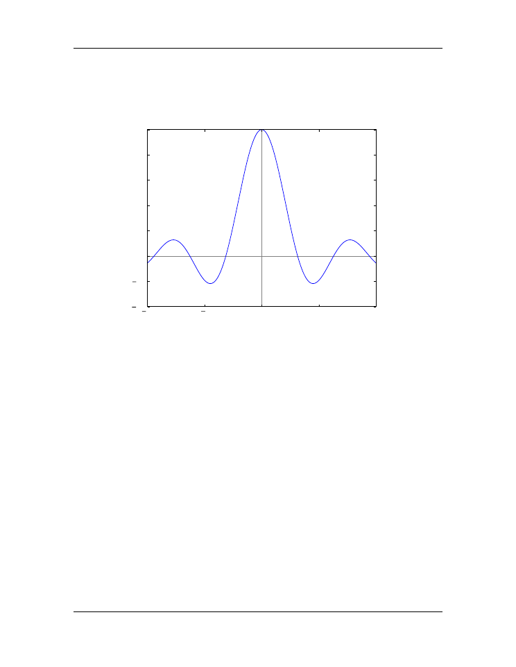
array. The code following the function definition plots
sinc
x
as a function of
x
.
In the program above, you may have noticed that the NumPy library is imported
after
the
sinc(x)
function definition. As the function uses the NumPy functions
sin
and
array
, you may wonder how this program can work. Doesn’t the
import numpy
statement have to be called before any NumPy functions are used? The answer it an em-
phatic “YES”. What you need to understand is that the function definition is
not executed
when it is defined, nor can it be as it has no input
x
data to process. That part of the code
is just a definition. The first time the code for the
sinc(x)
function is actually executed
is when it is called on line 14 of the program, which occurs after the NumPy library is
118
Chapter 7. Functions
Introduction to Python for Science, Release 0.9.23
imported in line 10. The figure below shows the plot of the
sinc
x
function generated by
the above code.
10
5
0
5
10
0.4
0.2
0.0
0.2
0.4
0.6
0.8
1.0
Figure 7.1: Plot of user-defined
sinc(x)
function.
7.1.2 Fast array processing in user-defined functions
While using loops to process arrays works just fine, it is usually not the best way to
accomplish the task in Python. The reason is that loops in Python are executed rather
slowly. To deal with this problem, the developers of NumPy introduced a number of
functions designed to process arrays quickly and efficiently. For the present case, what we
need is a conditional statement or function that can process arrays directly. The function
we want is called
where
and it is a part of the NumPy library. There
where
function
has the form
where(condition, output
if
True
, output
if
False
)
The first argument of the
where
function is a conditional statement involving an array.
The
where
function applies the condition to the array element by element, and returns the
second argument for those array elements for which the condition is
True
, and returns the
third argument for those array elements that are
False
. We can apply it to the
sinc(x)
function as follows
7.1. User-defined functions
119