ВУЗ: Не указан
Категория: Не указан
Дисциплина: Не указана
Добавлен: 17.04.2021
Просмотров: 3717
Скачиваний: 3

Introduction to Python for Science, Release 0.9.23
2.3.3 Tab completion
IPython also incorporates a number of shortcuts that make using the shell more efficient.
One of the most useful is
tab completion
. Let’s assume you have been following along
and that your are in the directory
Documents
or
My Documents
. To switch to the
directory
PyProgs
, you could type
cd PyProgs
. Instead of doing that, type
cd PyP
and then press the
TAB
key. This will complete the command, provided there is no ambi-
guity in how to finish the command. In the present case, that would mean that there was
no other subdirectory beginning with
PyP
. Tab completion works with any command you
type into the IPython terminal. Try it out! It will make your life more wonderful.
A related shortcut involves the
↑
key. If you type a command, say
cd
and then to press
the
↑
key, IPython will complete the
cd
command with the last instance of that command.
Thus, when you launch IPython, you can use this shortcut to take you to the directory you
used when you last ran IPython.
You can also simply press the
↑
key, which will simply recall the most recent command.
Repeated application of the
↑
key scrolls though the most recent commands in reverse
order. The
↓
key can be used to scroll in the other direction.
2.3.4 Recap of commands
Let’s recap the (magic) commands introduced above:
pwd
:
(
p
rint
w
orking
d
irectory) Prints the path of the current directory.
ls
:
(
l
i
s
t) Lists the names of the files and directories located in the current
directory.
mkdir
filename
:
(
m
a
k
e
dir
ectory) Makes a new directory
filename
.
cd
directoryname
:
(
c
hange
d
irectory) Changes the current directory to
di-
rectoryname
. Note: for this to work,
directoryname
must be a sub-
directory in the current directory. Typing
cd ~
changes to the home
directory of your computer. Typing
cd ..
moves the console one
directory up in the directory tree.
clear
:
Clears the IPython screen of previous commands.
run
filename
:
Runs (executes) a Python script. Described later in the sec-
tion
Tab completion:
Provides convenient shortcuts, with or without the arrow
keys, for executing commands in the IPython shell.
10
Chapter 2. Launching Python
Introduction to Python for Science, Release 0.9.23
2.4 Interactive Python as a calculator
You can use the IPython shell to perform simple arithmatic calculations. For example, to
find the product
3
×
15
, you type
3*15
at the
In
prompt and press
RETURN
:
In [1]:
3
*
15
Out[1]:
45
Python returns the correct product, as expected. You can do more complicated calcula-
tions:
In [2]:
6
+
21
/
3
Out[2]:
13.0
Let’s try some more arithmetic:
In [3]:
(
6
+
21
)
/
3
Out[3]:
9.0
Notice that the effect of the parentheses in
In [3]:
(6+21)/3
is to cause the ad-
dition to be performed first and then the division. Without the parentheses, Python will
always perform the multiplication and division operations
before
performing the addition
and subtraction operations. The order in which arithmetic operations are performed is the
same as for most calculators: exponentiation first, then multiplication or division, then
addition or subtraction, then left to right.
2.4.1 Binary arithmetic operations in Python
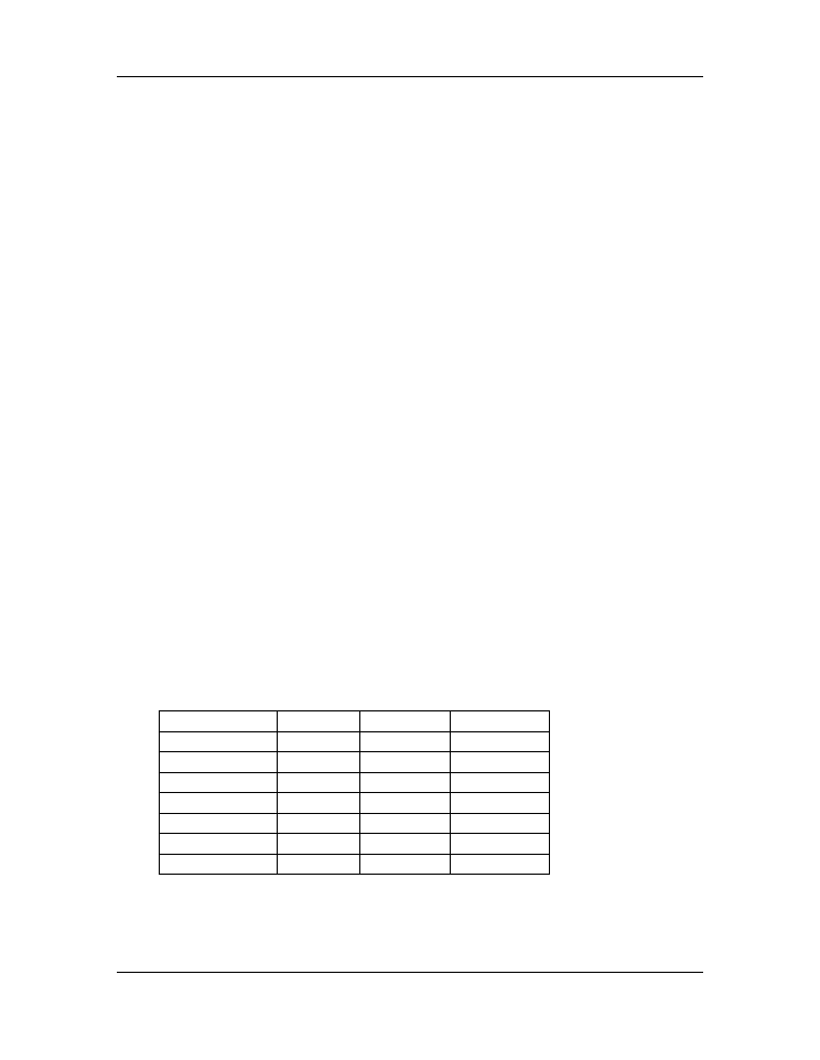
The table below lists the binary arithmatic operations in Python. It has all the standard
binary operators for arithmetic, plus a few you may not have seen before.
Operation
Symbol
Example
Output
addition
+
12+7
19
subtraction
-
12-7
5
multiplication
*
12*7
84
division
/
12/7
1.714285
floor division
//
12//7
1
remainder
%
12%7
5
exponentiation
**
12**7
35831808
“Floor division,” designated by the symbols
//
, means divide and keep only the integer
part without rounding. “Remainder,” designated by the symbols
%
, gives the remainder of
after a floor division.
2.4. Interactive Python as a calculator
11

Introduction to Python for Science, Release 0.9.23
2.4.2 Types of numbers
There are four different types of numbers in Python: plain integers, long integers, floating
point numbers, and complex numbers.
Plain integers
, or simply
integers
, are 32 bits (binary digits) long, which means they
extend from
−
2
31
=
−
2147483648
to
2
31
−
1 = 2147483647
. One bit is used to store
the sign of the integer so there are only 31 bits left—hence, the power of 31. In Python, a
number is automatically treated as an integer if is written without a decimal point and it
is within the bounds given above. This means that
23
, written without a decimal point,
is an integer and
23.
, written with a decimal point, is a floating point number. If an
integer extends beyond the bounds of a simple integer, the it becomes a
long integer
, and
is designated as such by an
L
following the last digit. Here are some examples of integer
arithmetic:
In [4]:
12
*
3
Out[4]:
36
In [5]:
4
+
5
*
6
-
(
21
*
8
)
Out[5]:
-
134
In [6]:
11
/
5
Out[6]:
2.2
In [7]:
11
//
5
Out[7]:
2
In [8]:
9734828
*
79372
# product of these two large integers
Out[8]:
772672768016L
# is a long integer
For the binary operators
+
,
-
,
*
, and
//
, the output is an integer if the inputs are integers.
The only exception is if the result of the calculation is out of the bounds of Python integers,
in which case Python automatically converts the result to a long integer. The output of
the division operator
/
is a floating point as of version 3 of Python. If an integer output is
desired when two integers are divided, the floor division operator
//
must be used. See
Important note on integer division in Python
Floating point
numbers are essentially rational numbers and can have a fractional part;
integers, by their very nature, have no fractional part. In most versions of Python running
on PCs or Macs, floating point numbers go between approximately
±
2
×
10
−
308
and
±
2
×
10
308
. Here are some examples of integer arithmetic:
In [9]:
12.
*
3.
Out[9]:
36.0
12
Chapter 2. Launching Python

Introduction to Python for Science, Release 0.9.23
In [10]:
123.4
*
(
-
53.9
)
/
sqrt(
5.
)
Out[10]:
-
2974.5338992050501
In [11]:
11.
/
5.
Out[11]:
2.2
In [12]:
11.
//
5.
Out[12]:
2.0
In [13]:
11.
%
5.
Out[13]:
1.0
In [14]:
6.022e23
*
300.
Out[14]:
1.8066e+26
Note that the result of any operation involving only floating point numbers as inputs is a
real number, even in the cases where the floor division
//
or remainder
%
operators are
used. The last output also illustrates an alternative way of writing floating point numbers
as a mantissa followed by and
e
or
E
followed by a power of 10: so 1.23e-12 is equivalent
to
1
.
23
×
10
−
12
.
We also sneaked into our calculations
sqrt
, the square root function. We will have more
to say about functions in a few pages.
Complex numbers
are written in Python as a sum of a real and imaginary part. For
example, the complex number
3
−
2
i
is represented as
3-2j
in Python where
j
represents
√
−
1
. Here are some examples of complex arithmetic:
In [15]:
(
2
+
3j
)
*
(
-
4
+
9j
)
Out[15]:
(
-
35
+
6j
)
In [16]:
(
2
+
3j
)
/
(
-
4
+
9j
)
Out[16]:
(
0.1958762886597938
-
0.3092783505154639j
)
In [17]:
sqrt(
-
3
)
Out[17]:
nan
In [18]:
sqrt(
-
3
+
0j
)
Out[18]:
1.7320508075688772j
Notice that to obtain the expected result or
√
−
3
, you must write the argument of the
square root function as a complex number. Otherwise, Python returns
nan
(not a number).
If you multiply an integer by a floating point number, the result is a floating point number.
Similarly, if you multiply a floating point number by a complex number, the result is a
2.4. Interactive Python as a calculator
13

Introduction to Python for Science, Release 0.9.23
complex number. Python always promotes the result to the most complex of the inputs.
2.4.3 Important note on integer division in Python
One peculiarity of all versions of Python prior to version 3 is that dividing two integers
by each other yields the “floor division” result—another integer. Therefore
3/2
yields
1
whereas
3./2
or
3/2.
or
3./2.
all yield
1.5
. Starting with version 3 of Python, all of
the above expressions, including
3/2
yield
1.5
. Unfortunately, we are using version 2.7
of Python so
3/2
yields
1
. You can force versions of Python prior to version 3 to divide
integers like version 3 does by typing
from __future__ import division
at
the beginning of an IPython session. You only need to type it once and it works for the
entire session.
2.5 Python Modules
The Python computer language consists of a “core” language plus a vast collection of
supplementary software that is contained in
modules
. Many of these modules come with
the standard Python distribution and provide added functionality for performing computer
system tasks. Other modules provide more specialized capabilities that not every user may
want. You can think of these modules as a kind of library from which you can borrow
according to your needs.
We will need three Python modules that are not part of the core Python distribution, but
are nevertheless widely used for scientific computing. The three modules are
NumPy
is the standard Python package for scientific computing with
Python. It provides the all-important
array
data structure, which
is at the very heart of NumPy. In also provides tools for creating
and manipulating arrays, including indexing and sorting, as well as
basic logical operations and element-by-element arithmetic operations
like addition, subtraction, multiplication, division, and exponentiation.
It includes the basic mathematical functions of trigonometry, expo-
nentials, and logarithms, as well vast collection of special functions
(Bessel functions,
etc.
), statistical functions, and random number gen-
erators.
It also includes a large number of linear algebra routines
that overlap with those in SciPy, although the SciPy routines tend to
be more complete. You can find more information about NumPy at
http://docs.scipy.org/doc/numpy/reference/index.html
14
Chapter 2. Launching Python