Файл: Курсовая работа по дисциплине Процессы и аппараты химической технологии на тему Adsorption.docx

5.5 Synthetic zeolites as engineered adsorbents

Zeolites occur in nature in high diversity. For practical applications, however, often synthetic zeolites are used. Synthetic zeolites can be manufactured from alkaline aqueous solutions of silicium and aluminum compounds under hydrothermal conditions. [18]

Zeolites are alum-silicates with the general formula (Me II, Me I 2) O ·Al₂O₃·n SiO₂ ·p H₂O. In the alum-silicate structure, tetrahedral AlO₄ and SiO₄ groups are connected via joint oxygen atoms. Zeolites are tectosilicates (framework silicates) with a porous structure characterized by windows and caves of defined sizes. Zeolites can be considered as derivatives of silicates where Si is partially substituted by Al. As a consequence of the different number of valence electrons of Si (4) and Al (3), the zeolite framework carries negative charges, which are compensated by metal cations. Depending on the molar SiO₂/Al₂O₃ ratio (modulus n), different classes can be distinguished – for instance, the well-known types A (n = 1.5…2.5), X (n = 2.2…3.0), and Y (n = 3.0…6.0). These classical zeolites are hydrophilic. They are in particular suitable for ion exchange processes (e.g., softening) but not for the adsorption of neutral organic substances. The hydrophobicity of zeolites increases with increasing modulus. High-silica zeolites with n > 10 are more hydrophobic and are therefore potential adsorbents for organic compounds. Although some promising experimental results for several organic adsorbates were published in the past, zeolites have not found broad application as adsorbents in water treatment until now. [16]

5.6 Natural and low-cost adsorbents

Among the natural and low-cost adsorbents, clay minerals have a special position. The application of natural clay minerals as adsorbents has been studied for a relatively long time. The adsorption properties of clay minerals or mineral mixtures such as bentonite (main component: montmorillonite) or Fuller’s earth (attapulgite and montmorillonite varieties) are related to the net negative charge of the mineral structure. This property allows clays to adsorb positively charged species – for instance, heavy metal cations such as Cu²⁺, Zn²⁺, or Cd²⁺. Relatively high adsorption capacities were also reported for organic dyes during treatment of textile wastewater. [17]

To improve the sorption capacity, clay minerals can be modified by organic cations to make them more organophilic. In recent decades, a growing interest in LCAs has been observed, and, in addition to clay, other potential adsorbents have gained increasing interest. This can be seen, for instance, from the strongly increasing number of published studies in this field. This ongoing development is driven by the fast industrial growth in some regions of the world (e.g., in Asia) accompanied by increasing environmental pollution and the search for low-cost solutions to these problems. In these regions, often natural materials as well as wastes from agricultural and industrial processes are available, which come into consideration as potential adsorbents. The scheme shown below illustrates the broad variety of possible LCAs. [15]

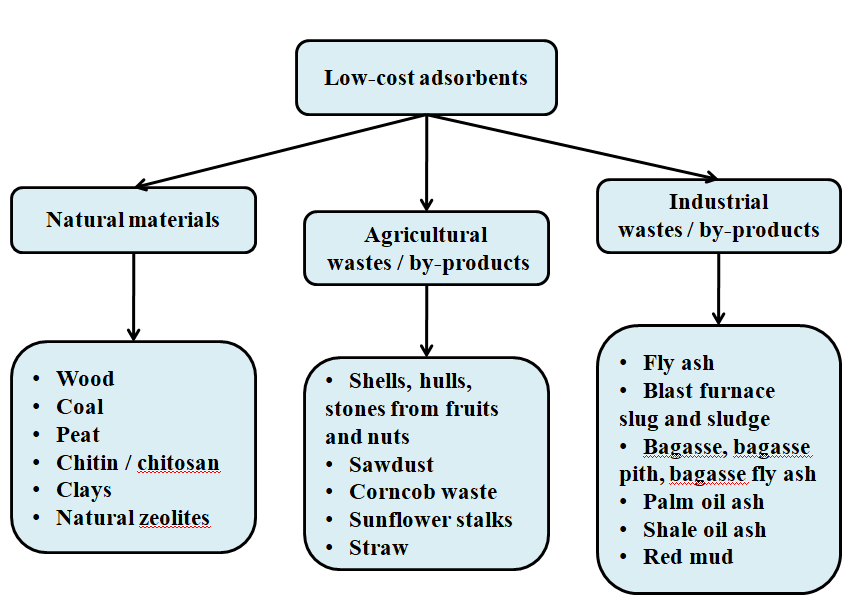
Figure 5.4 Selected low-cost adsorbents.
The adsorbents are mainly used untreated, but in some cases, physical and chemical pretreatment processes, such as heating or treatment with hydrolyzing chemicals, were also proposed. The studies on the adsorption properties of the alternative low-cost adsorbents were mainly directed to the removal of problematic pollutants from industrial wastewaters, in particular heavy metals from electroplating wastewaters and dyes from textile wastewaters. In some studies. phenols were also considered. Despite the increasing number of studies on the application of LCAs, there is still a lack of systematic investigations, including in-depth studies on the adsorption mechanisms on a strict theoretical basis, and also a lack of comparative studies under defined conditions. Therefore, it is not easy to evaluate the practical importance of the different alternative adsorbents for wastewater treatment. [20]

---

6 EXPERIMENTAL PART

6.1 Initial data for further calculations

Due to the fact that only the molar amounts of rising steam and flowing liquid remain the same along the height of the column (only their composition changes), it is advisable to carry out material calculations of the rectification process mainly in molar quantities. If the costs are set to be massive, then the concentration should be massive. The purpose of material balance equations‟ construction and solution is the identification of unknown material flows.
The content of ND in the mixture(mol fraction):

The molar concentration of the initial mixture :X_F = 0,38

Molar distillate concentration: X_d = 0,97

Molar concentration of the bottoms: X_W = 0,06

The pressure in the column is 1 atm.

Amount of starting mixture: F = 10000

The initial mixture is preheated to the boiling point. Provides for hot irrigation of the column.
Benzene and chloroform calculation:

The goal of composing and solving the equation of material balance is the definition of unknown material flows.

The boiling point of substances at P = 760 mmHg:

Benzene T _b.p.= 61,4 C;

Chloroform T _b.p.= 80,6 C.

Molecular masses of substances:

Benzene Mr = 78 kg/ kmol;

Chloroform Mr = 120 kg/ kmol.

We shall carry out the calculation by the method proposed in.

The equation of material balance has the form:

Where F is the flow rate of the initial mixture, kg/s;

D-top product consumption, kg/s;

W-consumption of the bottom product , kg/s;

-Corresponding mass fractions of the components, kg/kg.
Material balance calculation:

The goal of composing and solving the equation of material balance is to find of unknown material flows:

F = D + W

(1)

Where F – flow rate of the initial mixture, kg/s;

D – top product consumption, kg/s;

W – bottom product consumption, kg/s.
F • X_F = D • X_D + W • X_W (2)
Where F – flow rate of the initial mixture, kg/s;

D – top products consumption, kg/s;

W – bottom products consumption, kg/s;

X_F – molar concentration of the initial mixture;

X_D – molar concentration of the distillates;

X_W – molar concentration of the residue;
The molar consumption of raw material is defined by following formula:
G_F = F/M_F (3)
Where G_F – molar consumption of the initial mixture, kmol/h;

F - flow rate of the initial mixture, kg/s;

M_F – average molar weight, kg/mol.
The average molar weight is determined by below following formula:
M_F = M_C • X_F + M_B • (1 - X_F) (4)
Where M_F – average molar weight, kg/mol;

M_C – molar mass of the chloroform, kg/kmol;

M_B – molar mass of the benzene, kg/kmol;

X_F – molar concentration of the initial mixture.
M_F = 120 • 0,38 + 0,78 • (1 - 0,38) = 93,96 kg/mol.
The molar consumption:
G_F = F/M_f = 10000/93,96 = 106,42 kmol/h
The distillate flow:
G_D = G_F • ; kmol/h (5)
Where G_D – molar consumption of the distillates, kmol/h;

G_F – molar consumption of the initial mixture, kmol/h;

X_F – molar concentration of the initial mixture;

X_D – molar concentration of the distillates;

X_W – molar concentration of the residue.
G_D = 106,42 • = 37,42 kmol/h
The residue flow:
G_W = G_F – G_D (6)
Where G_W – molar consumption of the residue, kmol/h;

---

G_F – molar consumption of the initial mixture, kmol/h;

G_D – molar consumption of the distillates, kmol/h.
G_W = 106,42 - 37,42 = 69 kmol/h
F = D + W (7)
F = 37,42 + 69=106,42
Relatively molar flow of the feed:
F = (8)
Where F – relative molar flow of the feed, kmol/h;

X_F – molar concentration of the initial mixture, M;

X_D – molar concentration of the distillates, M;

X_W – molar concentration of the residue, M.
F = = 2,84 kmol/h
We calculate the material balance for each component.

How much chloroform in in kmol/h in the intial mixture:
F_C = G_F • X_F ; (9)
Where F_C – consumption of chloroform in the initial mixture, kmol/h;

G_F – molar consumption of the initial mixture, kmol/h;

X_F – molar concentration of the initial mixture, M.
F_C = 106,42  0,38 = 40,44 kmol/h
Let’s find the content of chloroform in the mixture in kg/h:
F_C’ = F_C • M_C (10)
Where F_C’ – consumption of chloroform in the initial mixture, kg/h;

F_C – consumption of chloroform in the initial mixture, kmol/h;

M_C – molar mass of the chloroform, kg/kmol.

Fc’ = 40,44  120 = 4852,8 kg/h
For benzene:
F_B = G_F • (1 - X_F) (11)
Where F_B – consumption of benzene in the initial mixture, kmol/h;

G_F – molar consumption of the initial mixture, kmol/h;

X_F – molar concentration of the initial mixture, M.
Fb = 106,42  (1 - 0,38) = 65,98 kmol/h
In kg/h:
F_B’ = F_B • M_B (12)
Where F_B’ – consumption of benzene in the initial mixture, kmol/h;

F_B – consumption of benzene in the initial mixture, kmol/h;

M_B – molar mass of the benzene, kg/kmol.
F_B’ = 66  78 = 5148 kg/h
Next , calculate how much chloroform will be:
D_C = G_D • X_D (13)
Where D_C – consumption of chloroform in the distillates, kmol/h;

G_D – molar consumption of the distillates, kmol/h;

X_D – molar concentration of the distillates, M.
D_C = 37,42  0,97 = 36,29 kmol/h
Also, in kg/h:
D_C’ = G_D • M_C (14)
Where D_C’ – consumption of chloroform in the distillates, kg/h;

G_D – molar consumption of the distillates, kmol/h;

M_C – molar mass of the chloroform, kg/kmol.
D_C’ = 36,29  120 = 4353,8 kg/h


Next, calculate the benzene:
D_B = G_D • (1 - X_D) (15)
Where D_B – consumption of benzene in the distillates, kmol/h;

G_D – molar consumption of the distillates, kmol/h;

X_D – molar concentration of the distillates, M.
D_B = 37,42 • (1-0,97) = 1,12 kmol/h
In kg/h:
D_B’ = D_B • M_B (16)
Where D_B’ – consumption of benzene in the distillates, kg/h;

D_B – consumption of benzene in the distillates, kmol/h;

M_B – molar mass of the benzene, kg/kmol.
D_B = 1,12 • 78 = 87,36 kg/h
How much chloroform in the residue:
W_C = G_W • X_W (17)
Where W_C – consumption of chloroform in the residues, kmol/h;

G_W – molar consumption of the residue, kmol/h;

X_W – molar concentration of the residue, M.
W_C = 69 • 0,06 = 4,14 kmol/h
In kg/h:
W_C’ = W_C • M_C (18)
Where W_C’ – consumption of chloroform in the residues, kg/h;

W_C – consumption of chloroform in the residues, kmol/h;

M_C – molar mass of the chloroform, kg/kmol.
W_C’ = 4,14 • 120 = 496,8 kg/h

---

How much benzene in the residue :
W_B = G_W • (1 - X_W) (19)
Where W_B – consumption of benzene in the residues, kmol/h;

G_W – molar consumption of the residue, kmol/h;

X_W – molar concentration of the residue, M.
W_B = 69 • (1 - 0,06) = 64,86 kmol/h
In kg/h:

W_B’ = W_B • M_B (20)
Where W_B’ – consumption of benzene in the residues, kg/h;

W_B – consumption of benzene in the residues, kmol/h;

M_B – molar mass of the chloroform, kg/kmol.
W_B’ = 64,86  78 = 5059,08 kg/h
Table 6.1 Table of material balance

Components	F		D		W
	Kg/h	Kmol/h	Kg/h	Kmol/h	Kg/h	Kmol/h
Chloroform	4852,8	40,44	4354,8	36,29	496,8	4,14
Benzene	5148	65,98	87,36	1,12	5059,08	64,86
Total	10000,8	106,42	4442,16	37,41	5555,88	69,26

2^nd experimental part.

Construction of the equilibrium and working lines and diagram

Determination of the working reflux ratio
In order to carry out further material calculations, it is required to construct the equilibrium lines of the t-x-y diagram.

Content of low-boiling and high-boiling components at various temperatures and pressures of 760 mmHg.

Atmosphere pressure:

P air = 760 mm.pm.cm

Pressure in the column

F = PK  P air = 1  760 = 760 mm.pm.cm
Table 6.2 Table of equilibrium composition

t , C	x	y
1	2	3
61,4	1	1
68,9	0,79	0,90
71,9	0,66	0,80
74,0	0,54	0,70
75,3	0,44	0,60
76,4	0,36	0,50
77,3	0,29	0,40

Extension of the table 6.2

1	2	3
78,2	0,22	0,30
79,0	0,15	0,20
79,8	0,08	0,10
80,6	0	0

---

The equilibrium curve the points of infection does not have. Determine the minimum number of phlegm.
R _min = (21)
Where X_D – molar concentration of the distillates, M;

X_F – molar concentration of the initial mixture, M;

Y_F – mole fraction of LBC in а vapor equilibrium with а liquid, M;

Y_f = 0,71 by diagram
R _min = = 0,78
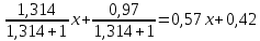
The working number phlegm is determined by the formula :
R = 1,3R_min + 0,3 (22)
Where R – working number of phlegm;

R_min – minimum number of phlegm.
R = 1,3  0,78 + 0,3 = 1,314
Equation for working lines:
а) for the top of the column:
y = (23)
R – working phlegm number.

y =
b) for the bottom:
y = (24)
Where R – working phlegm number;

X_W – molar concentration of the residue, M;

F – relative molar flow of the feed

y =

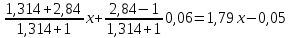
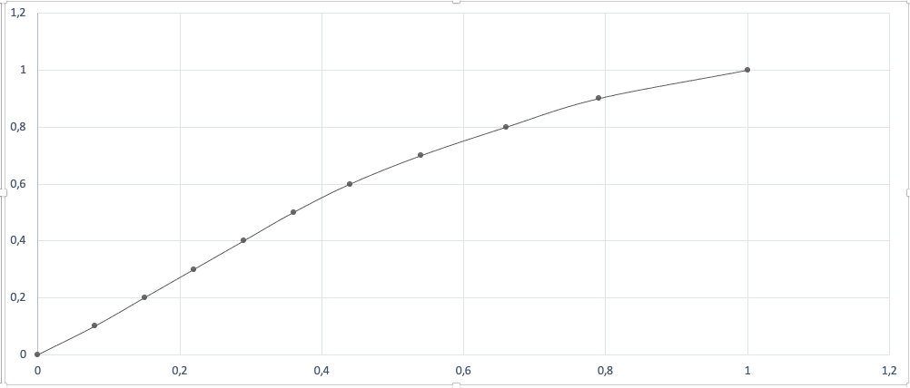
Figure 6.1 The equilibrium diagram of benzene-chloroform

---