ВУЗ: Не указан
Категория: Не указан
Дисциплина: Не указана
Добавлен: 17.04.2021
Просмотров: 3734
Скачиваний: 3

Introduction to Python for Science, Release 0.9.23
4.5 Exercises
1. Write a Python program that calculates how much money you can spend each day
for lunch for the rest of the month based on today’s date and how much money you
currently have in your lunch account. The program should ask you: (1) how much
money you have in your account, (2) what today’s date is, and (3) how many days
there are in month. The program should return your daily allowance. The results of
running your program should look like this:
How much money (in dollars) in your lunch account? 118.39
What day of the month is today? 17
How many days in this month? 30
You can spend $8.46 each day for the rest of the month.
Extra:
Create a dictionary (see
) that stores the number of days in each
month (forget about leap years) and have your program ask what month it is rather
than the number of days in the month.
2. From the IPython terminal, create the following three NumPy arrays:
a
=
array([
1
,
3
,
5
,
7
])
b
=
array([
8
,
7
,
5
,
4
])
c
=
array([
0
,
9
,
-
6
,
-
8
])
Now use the
zip
function to create the object
d
defined as
d
=
zip
(a, b, c)
d
out at the terminal prompt. What kind of object is
d
? Hint: It is not a NumPy
array. Convert
d
into a NumPy array and call that array
e
. Type
e
at the terminal
prompt so that
e
is printed out on the IPython terminal. One of the elements of
e
is
-8
. Show how to address and print out just that element of
e
. Show how to address
that same element of
d
. What has become of the three original arrays
a
,
b
, and
c
,
that is, how do they appear in
e
?
3. Create the following data file and then write a Python script to read it into a three
NumPy arrays with the variable names
f
,
a
,
da
for the frequency, amplitude, and
amplitude error.
Date:
2013
-
09
-
16
Data taken by Liam
and
Selena
frequency (Hz) amplitude (mm)
amp error (mm)
70
Chapter 4. Input and Output

Introduction to Python for Science, Release 0.9.23
0.7500
13.52
0.32
1.7885
12.11
0.92
2.8269
14.27
0.73
3.8654
16.60
2.06
4.9038
22.91
1.75
5.9423
35.28
0.91
6.9808
60.99
0.99
8.0192
33.38
0.36
9.0577
17.78
2.32
10.0962
10.99
0.21
11.1346
7.47
0.48
12.1731
6.72
0.51
13.2115
4.40
0.58
14.2500
4.07
0.63
Show that you have correctly read in the data by having your script print out to your
computer screen the three arrays. Format the printing so that it produces output like
this:
f
=
[
0.75
1.7885
2.8269
3.8654
4.9038
5.9423
6.9808
8.0192
9.0577
10.0962
11.1346
12.1731
13.2115
14.25
]
a
=
[
13.52
12.11
14.27
16.6
22.91
35.28
60.99
33.38
17.78
10.99
7.47
6.72
4.4
4.07
]
da
=
[
0.32
0.92
0.73
2.06
1.75
0.91
0.99
0.36
2.32
0.21
0.48
0.51
0.58
0.63
]
Note that the array
f
is displayed with four digits to the right of the decimal point
while the arrays
a
and
da
are displayed with only two. The columns of the dis-
played arrays need not line up as they do above.
4. Write a script to read the data from the previous problem into three NumPy arrays
with the variable names
f
,
a
,
da
for the frequency, amplitude, and amplitude error
and then, in the same script, write the data out to a data file, including the header,
with the data displayed in three columns, just as its displayed in the problem above.
It’s ok if the header lines begin with the
#
comment character. Your data file should
have the extension
.txt
.
5. Write a script to read the data from the previous problem into three NumPy arrays
with the variable names
f
,
a
,
da
for the frequency, amplitude, and amplitude error
and then, in the same script, write the data out to a csv data file, without the header,
to a data file with the data displayed in three columns. Use a single format specifier
4.5. Exercises
71

Introduction to Python for Science, Release 0.9.23
and set it to
"%0.16e"
. If you have access the spreadsheet program (like MS
Excel), try opening the file you have created with your Python script and verify that
the arrays are displayed in three columns. Note that your csv file should have the
extension
.csv
.
72
Chapter 4. Input and Output

CHAPTER
FIVE
PLOTTING
The graphical representation of data—plotting—is one of the most important tools for
evaluating and understanding scientific data and theoretical predictions. However, plot-
ting is not a part of core Python but is provided through one of several possible library
modules. The most highly developed and widely used plotting package for Python is
MatPlotLib (
http://MatPlotLib.sourceforge.net/
). It is a powerful and flexible program
that has become the
de facto
standard for 2-d plotting with Python.
Because MatPlotLib is an external library—in fact it’s a collection of libraries—it must
be imported into any routine that uses it. MatPlotLib makes extensive use of NumPy so
the two should be imported together. Therefore, for any program for which you would
like to produce 2-d plots, you should include the lines
import
numpy
as
np
import
matplotlib.pyplot
as
plt
There are other MatPlotLib sub-libraries, but the
pyplot
library provides nearly every-
thing that you need for 2-d plotting. The standard prefix for it is
plt
. MatPlotLib is auto-
matically loaded with the IPython shell so you do not need to use import matplotlib.pyplot
nor do you need to use the
plt
prefix when working in the IPython shell.
One final word before we get started: We only scratch the surface of what is possible using
MatPlotLib and as you become familiar with it, you will surely want to do more than this
manual describes. In that case, you need to go the the web to get more information. A
good place to start is
http://matplotlib.org/api/pyplot_summary.html
. Another interesting
web page is
http://matplotlib.org/gallery.html
73
Introduction to Python for Science, Release 0.9.23
5.1 An interactive session with
pyplot
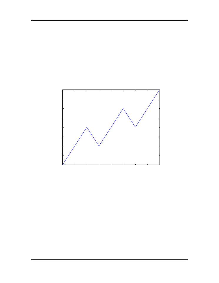
We begin with an interactive plotting session that illustrates some very basic features of
MatPlotLib. Type in the
plot
command shown below and press the return key. Take
care to follow the exact syntax.
In [1]:
plot([
1
,
2
,
3
,
2
,
3
,
4
,
3
,
4
,
5
])
Out[1]:
[
<
MatPlotLib
.
lines
.
Line2D at
0x94e1310
>
]
0
1
2
3
4
5
6
7
8
1.0
1.5
2.0
2.5
3.0
3.5
4.0
4.5
5.0
Figure 5.1: Interactive plot window
A window should appear with a plot that looks something like the
shown here. By default, the
plot
function draws a line between the data points that were
entered. You can save this plot to an image file by clicking on the floppy disk icon at the
top of the plot window. You can also zoom, pan, scroll through the plot, and return to the
original view using the other icons in the plot window. Experimenting with them reveals
their functions.
When you are finished, be sure to close the plot window.
Let’s take a closer look at the
plot
function. It is used to plot
x
-
y
data sets and is written
like this
74
Chapter 5. Plotting