ВУЗ: Не указан
Категория: Не указан
Дисциплина: Не указана
Добавлен: 17.04.2021
Просмотров: 3719
Скачиваний: 3

Introduction to Python for Science, Release 0.9.23
In [21]:
a
Out[21]:
array([ 0.859057
,
0.27228037,
0.87780026,
0.14341207,
0.05067356,
0.83490135,
0.54844515,
0.33583966,
0.31527767,
0.15868803])
In [22]:
a
.
sum()
# sum
Out[22]:
4.3963751104791005
In [23]:
a
.
mean()
# mean or average
Out[23]:
0.43963751104791005
In [24]:
a
.
var()
# variance
Out[24]:
0.090819477333711512
In [25]:
a
.
std()
# standard deviation
Out[25]:
0.30136270063448711
In [26]:
a
.
sort()
# sort small to large
In [27]:
a
Out[27]:
array([ 0.05067356,
0.14341207,
0.15868803,
0.27228037,
0.31527767,
0.33583966,
0.54844515,
0.83490135,
0.859057
,
0.87780026])
In [28]:
a
.
clip(
0.3
,
0.8
)
Out[29]:
array([ 0.3
,
0.3
,
0.3
,
0.3
,
0.31527767,
0.33583966,
0.54844515,
0.8
,
0.8
,
0.8
])
The
clip()
method provides an example of a method that takes an argument, in this
case the arguments are the lower and upper values to which array elements are cutoff if
their values are outside the range set by these values.
7.3 Example: linear least squares fitting
In this section we illustrate how to use functions and methods in the context of modeling
experimental data.
In science and engineering we often have some theoretical curve or
fitting function
that we
would like to fit to some experimental data. In general, the fitting function is of the form
130
Chapter 7. Functions
Introduction to Python for Science, Release 0.9.23
f
(
x
;
a, b, c, ...
)
, where
x
is the independent variable and
a
,
b
,
c
, ... are parameters to be
adjusted so that the function
f
(
x
;
a, b, c, ...
)
best fits the experimental data. For example,
suppose we had some data of the velocity
vs
time for a falling mass. If the mass falls
only a short distance such that its velocity remains well below its terminal velocity, we
can ignore air resistance. In this case, we expect the acceleration to be constant and the
velocity to change linearly in time according to the equation
v
(
t
) =
v
0
−
gt ,
(7.1)
where
g
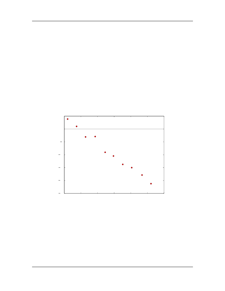
is the local gravitational acceleration. We can fit the data graphically, say by
plotting it as shown below in Fig.
and then drawing a line through the data. When
we draw a straight line through a data, we try to minimize the distance between the points
and the line, globally averaged over the whole data set.
0.0
0.5
1.0
1.5
2.0
2.5
3.0
time (s)
25
20
15
10
5
0
5
velocity (m/s)
Least squares fit w/o uncertainties
v0 = 4.4 m/s
a = -9.8 m/s^2
redchisq = 0.84
Figure 7.2: Velocity
vs
time for falling mass.
While this can give a reasonable estimate of the best fit to the data, the procedure is rather
ad hoc
. We would prefer to have a more well-defined analytical method for determining
what constitutes a “best fit”. One way to do that is to consider the sum
S
=
n
X
i
[
y
i
−
f
(
x
i
;
a, b, c, ...
)]
2
,
(7.2)
7.3. Example: linear least squares fitting
131


Introduction to Python for Science, Release 0.9.23
where
y
i
and
f
(
x
i
;
a, b, c, ...
)
are the values of the experimental data and the fitting func-
tion, respectively, at
x
i
, and
S
is the square of their difference summed over all
n
data
points. The quantity
S
is a sort of global measure of how much the the fit
f
(
x
i
;
a, b, c, ...
)
differs from the experimental data
y
i
.
Notice that for a given set of data points
{
x
i
, y
i
}
,
S
is a function only of the fitting
parameters
a, b, ...
, that is,
S
=
S
(
a, b, c, ...
)
. One way of defining a
best
fit, then, is to
find the values of the fitting parameters
a, b, ...
that minimize the
S
.
In principle, finding the values of the fitting parameters
a, b, ...
that minimize the
S
is a
simple matter. Just set the partial derivatives of
S
with respect to the fitting parameter
equal to zero and solve the resulting system of equations:
∂S
∂a
= 0
,
∂S
∂b
= 0
, ...
(7.3)
Because there are as many equations as there are fitting paramters, we should be able to
solve the system of equations and find the values of the fitting parameters that minimize
S
.
Solving those systems of equations is straightforward if the fitting function
f
(
x
;
a, b, ...
)
is linear in the fitting parameters. Some examples of fitting functions linear in the fitting
parameters are:
f
(
x
;
a, b
) =
a
+
bx
f
(
x
;
a, b, c
) =
a
+
bx
+
cx
2
f
(
x
;
a, b, c
) =
a
sin
x
+
be
x
+
ce
−
x
2
.
(7.4)
For fitting functions such as these, taking the partial derivatives with respect to the fitting
parameters, as proposed in (
), results in a set of algebraic equations that are linear in
the fitting paramters
a, b, ...
Because they are linear, these equations can be solved in a
straightforward manner.
For cases in which the fitting function is not linear in the fitting parameters, one can
generally still find the values of the fitting parameters that minimize
S
but finding them
requires more work, which goes beyond our immediate interests here.
7.3.1 Linear regression
We start by considering the simplest case, fitting a straight line to a data set, such as the
one shown in Fig.
above. Here the fitting function is
f
(
x
) =
a
+
bx
, which is linear
in the fitting parameters
a
and
b
. For a straight line, the sum in (
) becomes
S
(
a, b
) =
X
i
(
y
i
−
a
−
bx
i
)
2
.
(7.5)
132
Chapter 7. Functions

Introduction to Python for Science, Release 0.9.23
Finding the best fit in this case corresponds to finding the values of the fitting parameters
a
and
b
for which
S
(
a, b
)
is a minimum. To find the minimum, we set the derivatives of
S
(
a, b
)
equal to zero:
∂S
∂a
=
X
i
−
2(
y
i
−
a
−
bx
i
) = 2
na
+
b
X
i
x
i
−
X
i
y
i
!
= 0
∂S
∂b
=
X
i
−
2(
y
i
−
a
−
bx
i
)
x
i
= 2
a
X
i
x
i
+
b
X
i
x
2
i
−
X
i
x
i
y
i
!
= 0
(7.6)
Dividing both equations by
2
n
leads to the equations
a
+
b
¯
x
= ¯
y
a
¯
x
+
b
1
n
X
i
x
2
i
=
1
n
X
i
x
i
y
i
(7.7)
where
¯
x
=
1
n
X
i
x
i
¯
y
=
1
n
X
i
y
i
.
(7.8)
Solving Eq. (
) for the fitting parameters gives
b
=
P
i
x
i
y
i
−
n
¯
x
¯
y
P
i
x
2
i
−
n
¯
x
2
a
= ¯
y
−
b
¯
x .
(7.9)
Noting that
n
¯
y
=
P
i
y
and
n
¯
x
=
P
i
x
, the results can be written as
b
=
P
i
(
x
i
−
¯
x
)
y
i
P
i
(
x
i
−
¯
x
)
x
i
a
= ¯
y
−
b
¯
x .
(7.10)
While Eqs. (
) are equivalent analytically, Eq. (
) is preferred for numer-
ical calculations because Eq. (
) is less sensitive to roundoff errors. Here is a Python
function implementing this algorithm:
1
def
LineFit
(x, y):
2
’’’ Returns slope and y-intercept of linear fit to (x,y)
3
data set’’’
7.3. Example: linear least squares fitting
133

Introduction to Python for Science, Release 0.9.23
4
xavg
=
x
.
mean()
5
slope
=
(y
*
(x
-
xavg))
.
sum()
/
(x
*
(x
-
xavg))
.
sum()
6
yint
=
y
.
mean()
-
slope
*
xavg
7
return
slope, yint
It’s hard to imagine a simpler implementation of the linear regression algorithm.
7.3.2 Linear regression with weighting:
χ
2
The linear regression routine of the previous section weights all data points equally. That
is fine if the absolute uncertainty is the same for all data points. In many cases, however,
the uncertainty is different for different points in a data set. In such cases, we would like
to weight the data that has smaller uncertainty more heavily than those data that have
greater uncertainty. For this case, there is a standard method of weighting and fitting data
that is known as
χ
2
(or
chi-squared
) fitting. In this method we suppose that associated
with each
(
x
i
, y
i
)
data point is an uncertainty in the value of
y
i
of
±
σ
i
. In this case, the
“best fit” is defined as the the one with the set of fitting parameters that minimizes the
sum
χ
2
=
X
i
y
i
−
f
(
x
i
)
σ
i
2
.
(7.11)
Setting the uncertainties
σ
i
= 1
for all data points yields the same sum
S
we introduced
in the previous section. In this case, all data points are weighted equally. However, if
σ
i
varies from point to point, it is clear that those points with large
σ
i
contribute less to the
sum than those with small
σ
i
. Thus, data points with large
σ
i
are weighted less than those
with small
σ
i
.
To fit data to a straight line, we set
f
(
x
) =
a
+
bx
and write
χ
2
(
a, b
) =
X
i
y
i
−
a
−
bx
i
σ
i
2
.
(7.12)
Finding the minimum for
χ
2
(
a, b
)
follows the same procedure used for finding the mini-
mum of
S
(
a, b
)
in the previous section. The result is
b
=
P
i
(
x
i
−
ˆ
x
)
y
i
/σ
2
i
P
i
(
x
i
−
ˆ
x
)
x
i
/σ
2
i
a
= ˆ
y
−
b
ˆ
x .
(7.13)
134
Chapter 7. Functions