ВУЗ: Не указан
Категория: Не указан
Дисциплина: Не указана
Добавлен: 17.04.2021
Просмотров: 3732
Скачиваний: 3

Introduction to Python for Science, Release 0.9.23
23.21
-55
10
5. Modify the function
LineFitWt(x, y)
you wrote in Exercise 4 above so that in
addition to returning the fitting parameters
a
and
b
, it also returns the uncertainties
in the fitting parameters
σ
a
and
σ
b
using the formulas given by Eq. (
). Use
your new fitting function to find the uncertainties in the fitted slope and
y
-intercept
for the data provided with Exercise 4.
140
Chapter 7. Functions

CHAPTER
EIGHT
CURVE FITTING
One of the most important tasks in any experimental science is modeling data and de-
termining how well some theoretical function describes experimental data. In the last
chapter, we illustrated how this can be done when the theoretical function is a simple
straight line in the context of learning about Python functions and methods. Here we
show how this can be done for a arbitrary fitting functions, including linear, exponential,
power law, and other nonlinear fitting functions.
8.1 Using linear regression for fitting non-linear
functions
We can use our results for linear regression with
χ
2
weighting that we developed in Chap-
ter 7 to fit functions that are nonlinear in the fitting parameters,
provided
we can transform
the fitting function into one that is linear in the fitting parameters and in the independent
variable (
x
).
8.1.1 Linear regression for fitting an exponential function
To illustrate this approach, let’s consider some experimental data taken from a radioactive
source that was emitting beta particles (electrons). We notice that the number of elec-
trons emitted per unit time is decreasing with time. Theory suggests that the number of
electrons
N
emitted per unit time should decay exponentially according to the equation
N
(
t
) =
N
0
e
−
t/τ
.
(8.1)
141

Introduction to Python for Science, Release 0.9.23
This equation is nonlinear in
t
and in the fitting parameter
τ
and thus cannot be fit using
the method of the previous chapter. Fortunately, this is a special case for which the fitting
function can be transformed into a linear form. Doing so will allow us to use the fitting
routine we developed for fitting linear functions.
We begin our analysis by transforming our fitting function to a linear form. To this end
we take the logarithm of Eq. (
ln
N
= ln
N
0
−
t
τ
.
With this tranformation our fitting function is linear in the independent variable
t
. To
make our method work, however, our fitting function must be linear in the
fitting param-
eters
, and our transformed function is still nonlinear in the fitting parameters
τ
and
N
0
.
Therefore, we define new fitting parameters as follows
a
= ln
N
0
b
=
−
1
/τ
(8.2)
Now if we define a new dependent variable
y
= ln
N
, then our fitting function takes the
form of a fitting function that is linear in the fitting parameters
a
and
b
y
=
a
+
bx
where the independent variable is
x
=
t
and the dependent variable is
y
= ln
N
.
We are almost ready to fit our transformed fitting function, with transformed fitting pa-
rameters
a
and
b
, to our transformed independent and dependent data,
x
and
y
. The last
thing we have to do is to transform the estimates of the uncertainties
δN
in
N
to the un-
certainties
δy
in
y
(= ln
N
)
. So how much does a given uncertainty in
N
translate into an
uncertainty in
y
? In most cases, the uncertainty in
y
is much smaller than
y
,
i.e.
δy
y
;
similarly
δN
N
. In this limit we can use differentials to figure out the relationship
between these uncertainties. Here is how it works for this example:
y
= ln
N
δy
=
∂y
∂N
δN
δy
=
δN
N
.
(8.3)
Equation (
) tells us how a small change
δN
in
N
produces a small change
δy
in
y
. Here
we identify the differentials
dy
and
dN
with the uncertainties
δy
and
δN
. Therefore, an
uncertainty of
δN
in
N
corresponds, or translates, to an uncertainty
δy
in
y
.
142
Chapter 8. Curve Fitting

Introduction to Python for Science, Release 0.9.23
Let’s summarize what we have done so far. We started with the some data points
{
t
i
, N
i
}
and some addition data
{
δN
i
}
where each datum
δN
i
corresponds to the uncertainty in
the experimentally measured
N
i
. We wish to fit these data to the fitting function
N
(
t
) =
N
0
e
−
t/τ
.
We then take the natural logarithm of both sides and obtain the linear equation
ln
N
= ln
N
0
−
t
τ
y
=
a
+
bx
(8.4)
with the obvious correspondences
x
=
t
y
= ln
N
a
= ln
N
0
b
=
−
1
/τ
(8.5)
Now we can use the linear regression routine with
χ
2
weighting that we developed in the
previous section to fit (
) to the transformed data
x
i
(=
t
i
)
and
y
i
(= ln
N
i
)
. The inputs
are the tranformed data
x
i
, y
i
, δy
i
. The outputs are the fitting parameters
a
and
b
, as well
as the estimates of their uncertainties
δa
and
δb
along with the value of
χ
2
. You can obtain
the values of the original fitting parameters
N
0
and
τ
by taking the differentials of the last
two equations in Eq. (
δa
=
∂a
∂N
0
δN
0
=
δN
0
N
0
δb
=
∂b
∂τ
δτ
=
δτ
τ
2
(8.6)
The Python routine below shows how to implement all of this for a set of experimental
data that is read in from a data file.
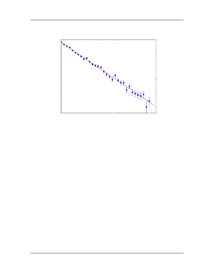
Figure
shows the output of the fit to simulated beta decay data obtained using the
program below. Note that the error bars are large when the number of counts
N
are
small. This is consistent with what is known as
shot noise
(noise that arises from counting
discrete events), which obeys
Poisson
statistics. You will study sources of noise, including
shot noise, later in your lab courses. The program also prints out the fitting parameters of
the transformed data as well as the fitting parameters for the exponential fitting function.
import
numpy
as
np
import
matplotlib.pyplot
as
plt
8.1. Using linear regression for fitting non-linear functions
143
Introduction to Python for Science, Release 0.9.23
0
20
40
60
80
100
t
2
3
4
5
6
7
ln(N)
A = ln N0 = 6.79
±
0.02
B = -1/tau = 0.0481
±
0.0007
χ
2
r
= 0.996
N0 = 892
±
16
tau = 20.8
±
0.3 days
Fit to : ln
N
=
−
t/τ
+ln
N
0
Figure 8.1: Semi-log plot of beta decay measurements from Phosphorus-32.
def
LineFitWt
(x, y, sig):
"""
Fit to straight line.
Inputs: x and y arrays and uncertainty array (unc) for y data.
Ouputs: slope and y-intercept of best fit to data.
"""
sig2
=
sig
**
2
norm
=
(
1.
/
sig2)
.
sum()
xhat
=
(x
/
sig2)
.
sum()
/
norm
yhat
=
(y
/
sig2)
.
sum()
/
norm
slope
=
((x
-
xhat)
*
y
/
sig2)
.
sum()
/
((x
-
xhat)
*
x
/
sig2)
.
sum()
yint
=
yhat
-
slope
*
xhat
sig2_slope
=
1.
/
((x
-
xhat)
*
x
/
sig2)
.
sum()
sig2_yint
=
sig2_slope
*
(x
*
x
/
sig2)
.
sum()
/
norm
return
slope, yint, np
.
sqrt(sig2_slope), np
.
sqrt(sig2_yint)
def
redchisq
(x, y, dy, slope, yint):
chisq
=
(((y
-
yint
-
slope
*
x)
/
dy)
**
2
)
.
sum()
return
chisq
/
float
(x
.
size
-
2
)
# Read data from data file
144
Chapter 8. Curve Fitting