ВУЗ: Не указан
Категория: Не указан
Дисциплина: Не указана
Добавлен: 17.04.2021
Просмотров: 3730
Скачиваний: 3

Introduction to Python for Science, Release 0.9.23
where
ˆ
x
=
P
i
x
i
/σ
2
i
P
i
1
/σ
2
i
ˆ
y
=
P
i
y
i
/σ
2
i
P
i
1
/σ
2
i
.
(7.14)
For a fit to a straight line, the overall quality of the fit can be measured by the reduced
chi-squared parameter
χ
2
r
=
χ
2
n
−
2
(7.15)
where
χ
2
is given by Eq. (
) evaluated at the optimal values of
a
and
b
given by
Eq. (
). A good fit is characterized by
χ
2
r
≈
1
. This makes sense because if the
uncertainties
σ
i
have been properly estimated, then
[
y
i
−
f
(
x
i
)]
2
should on average be
roughly equal to
σ
2
i
, so that the sum in Eq. (
) should consist of
n
terms approximately
equal to 1. Of course, if there were only 2 terms (
n=2
), then
χ
2
would be zero as the best
straight line fit to two points is a perfect fit. That is essentially why
χ
2
r
is normalized
using
n
−
2
instead of
n
. If
χ
2
r
is significantly greater than 1, this indicates a poor fit to
the fitting function (or an underestimation of the uncertainties
σ
i
). If
χ
2
r
is significantly
less than 1, then it indicates that the uncertainties were probably overestimated (the fit and
fitting function may or may not be good).
We can also get estimates of the uncertainties in our determination of the fitting parame-
ters
a
and
b
, although deriving the formulas is a bit more involved that we want to get into
here. Therefore, we just give the results:
σ
2
b
=
1
P
i
(
x
i
−
ˆ
x
)
x
i
/σ
2
i
σ
2
a
=
σ
2
b
P
i
x
2
i
/σ
2
i
P
i
1
/σ
2
i
.
(7.16)
The estimates of uncertainties in the fitting parameters depend explicitly on
{
σ
i
}
and will
only be meaningful if (
i
)
χ
2
r
≈
1
and (
ii
) the estimates of the uncertainties
σ
i
are accurate.
You can find more information, including a derivation of Eq. (
), in
Data Reduction
and Error Analysis for the Physical Sciences, 3rd ed
by P. R. Bevington & D. K. Robin-
son, McGraw-Hill, New York, 2003.
7.3. Example: linear least squares fitting
135
Introduction to Python for Science, Release 0.9.23
0.0
0.5
1.0
1.5
2.0
2.5
3.0
time (s)
25
20
15
10
5
0
5
velocity (m/s)
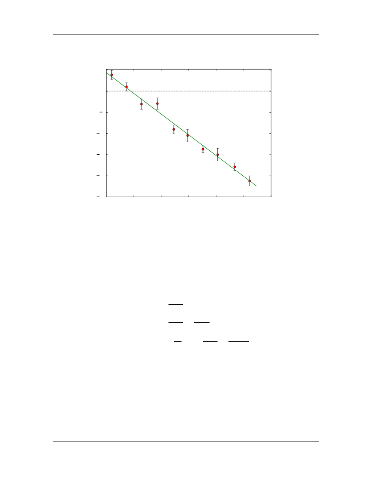
Least squares fit w/o uncertainties
v0 = 4.4 m/s
a = -9.8 m/s^2
redchisq = 0.84
a = 4.4 ± 0.7 m/s
b = -9.8 ± 0.4 m/s
2
χ
2
= 0.839
Fit to y = ax + b
Figure 7.3: Fit using
χ
2
least squares fitting routine with data weighted by error bars.
7.4 Exercises
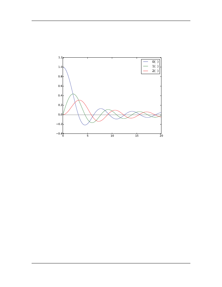
1. Write a function that can return each of the first three spherical Bessel functions
j
n
(
x
)
:
j
0
(
x
) =
sin
x
x
j
1
(
x
) =
sin
x
x
2
−
cos
x
x
j
2
(
x
) =
3
x
2
−
1
sin
x
x
−
3 cos
x
x
2
(7.17)
Your function should take as arguments a NumPy array
x
and the order
n
, and
should return an array of the designated order
n
spherical Bessel function. Take
care to make sure that your functions behave properly at
x
= 0
.
Demonstrate the use of your function by writing a Python routine that plots the
three Bessel functions for
0
≤
x
≤
20
. Your plot should look like the one below.
Something to think about: You might note that
j
1
(
x
)
can be written in terms of
j
0
(
x
)
, and that
j
2
(
x
)
can be written in terms of
j
1
(
x
)
and
j
0
(
x
)
. Can you take
136
Chapter 7. Functions
Introduction to Python for Science, Release 0.9.23
advantage of this to write a more efficient function for the calculations of
j
1
(
x
)
and
j
2
(
x
)
?
x
j x
j x
j x
2.
(a) Write a function that simulates the rolling of
n
dice. Use the NumPy function
random.random_integers(6)
, which generates a random integer be-
tween 1 and 6 with equal probability (like rolling fair dice). The input of your
function should be the number of dice thrown each roll and the output should
be the sum of the
n
dice.
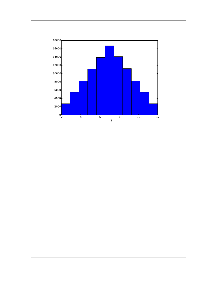
(b) “Roll” 2 dice 10,000 times keeping track of all the sums of each set of
rolls in a list.
Then use your program to generate a histogram summa-
rizing the rolls of two dice 10,000 times.
The result should look like
the histogram plotted below.
Use the MatPlotLib function
hist
(see
http://matplotlib.org/api/pyplot_summary.html
) and set the number of bins in
the histogram equal to the number of different possible outcomes of a roll of
your dice. For example, the sum of two dice can be anything between 2 and
12, which corresponds to 11 possible outcomes. You should get a histogram
that looks like the one below.
(c) “Repeat part (b) using 3 dice and plot the resulting histogram.
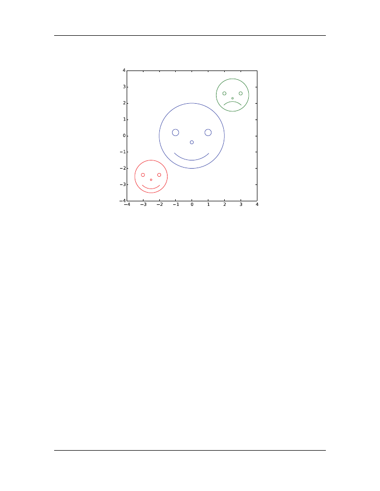
3. Write a function to draw a circular smiley face with eyes, a nose, and a mouth.
One argument should set the overall size of the face (the circle radius). Optional
arguments should allow the user to specify the
(
x, y
)
position of the face, whether
7.4. Exercises
137
Introduction to Python for Science, Release 0.9.23
sum of dice
the face is smiling or frowning, and the color of the lines. The default should
be a smiling blue face centered at
(0
,
0)
. Once you write your function, write
a program that calls it several times to produce a plot like the one below (cre-
ative improvisation is encouraged!). In producing your plot, you may find the call
plt.axes().set_aspect(1)
useful so that circles appear as circles and not
ovals. You should only use MatPlotLib functions introduced in this text. To create
a circle you can create an array of angles that goes from 0 to
2
π
and then produce
the
x
and
y
arrays for your circle by taking the cosine and sine, respectively, of the
array. Hint: You can use the same
(
x, y
)
arrays to make the smile and frown as you
used to make the circle by plotting appropriate slices of those arrays. You do not
need to create new arrays.
4. In the section
Example: linear least squares fitting
, we showed that the best fit of a
line
y
=
a
+
bx
to a set of data
{
(
x
i
, y
i
)
}
is obtained for the values of
a
and
b
given
by Eq. (
). Those formulas were obtained by finding the values of
a
and
b
that
minimized the sum in Eq. (
). This approach and these formulas are valid when
the uncertainties in the data are the same for all data points. The Python function
LineFit(x, y)
in the section
Example: linear least squares fitting
implements
Eq. (
(a) Write a new fitting function
LineFitWt(x, y)
that implements the for-
mulas given in Eq. (
) that minimize the
χ
2
function give by Eq. (
This more general approach is valid when the individual data points have dif-
138
Chapter 7. Functions
Introduction to Python for Science, Release 0.9.23
ferent weightings
or
when they all have the same weighting. You should also
write a function to calculate the reduced chi-squared
χ
2
r
defined by Eq. (
(b) Write a Python program that reads in the data below, plots it, and fits it us-
ing the two fitting functions
LineFit(x, y)
and
LineFitWt(x, y)
.
Your program should plot the data with error bars and with
both
fits with
and without weighting, that is from
LineFit(x, y)
and
LineFitWt(x,
y, dy)
. It should also report the results for both fits on the plot, similar to
the output of the supplied program above, as well as the values of
χ
2
r
, the re-
duce chi-squared value, for both fits. Explain why weighting the data gives a
steeper or less steep slope than the fit without weighting.
Velocity vs time data
for a falling mass
time (s)
velocity (m/s)
uncertainty (m/s)
2.23
139
16
4.78
123
16
7.21
115
4
9.37
96
9
11.64
62
17
14.23
54
17
16.55
10
12
18.70
-3
15
21.05
-13
18
7.4. Exercises
139