Файл: В. И. Ульянова (Ленина) (СПбгэту лэти) Направление 27. 04. 04 Управление в технических системах Магистерская программа.docx
ВУЗ: Не указан
Категория: Не указан
Дисциплина: Не указана
Добавлен: 25.10.2023
Просмотров: 282
Скачиваний: 1
СОДЕРЖАНИЕ
1.1 Explaining neural network:
1.2 Explaining the functionality of Neural Networks Works:
1.3.1 Convolutional Neural networks (CNN):
2. DESIGNING A CONVOLUTIONAL NEURAL NETWORK
2.1 Recurrent neural networks (RNNs):
2.2 Understanding Long Short-Term Memory (LSTM):
2.3 Describing LSTM mathematically:
2.4 Recurrent neural networks functionality in voice cloning applications:
3. IMPROVING DEEP LEARNING NETWORKS
3.1 Structure of Deep Learning:
3.2 Natural Language Processing using Voice Data:
4. VOICE PRE-PROCESSING USING DEEP LEARNING
4.2 Voice preprocessing implementation and logic:
4.3 Fast Fourier Transform (FFT):
4.4 Short-Time Fourier-Transform (STFT):
4.5 Mel frequency spectrum (MFCC):
4.7.3 Budling the autoencoder:
4.7.5 Results of the training process:
5.1 Explaining text to speech models (TTS):
5.2 DALL-E and its functionality:
5.3 Denoising Diffusion Probabilistic Models (DDPMs) and its functionality:
5.6 Implementing Tortoise-TTS:
5.6.2 Fine-Tuning Tortoise-TTS Model:
5.6.4 Installing Tortoise-TTS:
6.1 Compartment and validation of voice cloning output data:
7.2 Object and Company Description:
7.3 Market Analysis (Russia, Saint Petersburg):
7.4 Market Size and Growth Potential:
7.7 Marketing and Distribution Channels:
7.8 Regulatory and Cultural Considerations:
7.10 Economic Result Estimation:
7.11 Financial and Funding Plan:
Deep learning has shown tremendous success in a variety of applications such as computer vision, speech recognition, natural language processing, and robotics. The capacity of deep learning to automatically learn hierarchical representations of the data allows it to extract complicated patterns and characteristics that are challenging to extract using conventional machine learning techniques. This is one of deep learning's main advantages.
Deep learning employs a variety of neural network types, such as feedforward neural networks, recurrent neural networks, and convolutional neural networks. The most basic sort of neural network is a feedforward network, which is made up of numerous layers of nodes coupled in a forward direction. Regression and classification issues are frequently addressed by these networks.
1.1 Explaining neural network:
Neural networks are computational models that mimic the behavior of the human brain by using interconnected nodes, also known as artificial neurons, to process information. These nodes are arranged in layers and connected to each other through weights that are adjusted during the training process. The input layer receives information from the outside world, and the output layer produces the network's final output. In between the input and output layers, there can be one or more hidden layers where complex transformations take place. Each neuron in the network calculates a weighted sum of its inputs, applies an activation function to it, and then passes the result to the next layer. If the output of a neuron exceeds a certain threshold, it becomes active and sends its output to the next layer. By adjusting the weights and biases of the neurons during training, neural networks can learn to recognize patterns in data and make predictions.
Neural networks use training data to gain knowledge and improve their accuracy over time. It is possible to swiftly classify and aggregate data using these learning algorithms once they have been refined. They are crucial tools in computer science and artificial intelligence. Speech and picture recognition tasks can be completed in minutes rather than hours when compared to manual identification by human experts. One of the most well-known neural networks is the one used in the Google search engine.
1.2 Explaining the functionality of Neural Networks Works:
It is considered that each node is assumed to have its own linear regression model, which includes input data, weights, slope (or limit), and outputs. The formula will be as follows in equations 1 and 2:


When the input layer is selected, the weights are assigned. The greatest weight contributes more to the output than the other weights, which makes it easier to assess the importance of any particular variable. The inputs are then multiplied by their corresponding weights and added together. The activation function then receives the output and selects the output to use. The node is "launched" (or activated), and data is sent to the network's next tier, if these outputs go over the set limit. As a result, the outputs of one node become the inputs of the subsequent node. Since information is transmitted from one layer to the next, this neural network is a feed-forward network.
1.3 Types of neural networks:
There are various forms of neural networks, each of which serves a particular function. The following are the most frequent neural network types that you might encounter due to their widespread use, though this is not an exhaustive list:
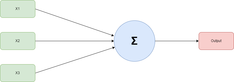
The receiver is the first class of neural network, developed by Frank Rosenblatt in 1958. It is the most basic kind of neural network, consisting of just one neuron:

Figure 1:Receiver neural network.
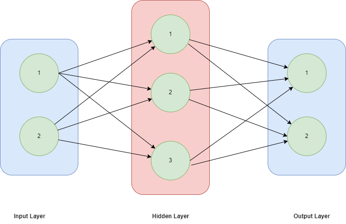
It focuses mostly on feed-forward neural networks, also called MLPs. The structure consists of an input layer, a hidden layer or levels, and an output layer. Because most real-world events aren't linear, even though these neural networks are frequently referred to as MLPs, it's important to keep in mind that they are actually composed of sigmoid neurons rather than receptors.
These models serve as the building blocks for neural networks used in computer vision, natural language processing, and other fields. They are typically fed training data.

Figure 2: Feed forward neural network.
1.3.1 Convolutional Neural networks (CNN):
CNNs are similar to feed-forward networks, however they are more frequently used for computer vision, image recognition, and/or model recognition. These networks employ methods from linear algebra, notably matrix multiplication, to find patterns in the image.
Deep learning models known as convolutional neural networks (CNNs) are frequently employed in computer vision tasks like segmentation, object detection, and image categorization. Because of their ability to automatically learn characteristics from input images, CNNs are the best choice for applications where manually extracting features would be challenging or time-consuming.
The convolutional layer is a CNN's fundamental building piece. In this layer, a collection of filters (also known as kernels) is applied to the input image to produce a set of feature maps by convolving the image with the filter weights. Each feature map draws attention to a particular pattern or aspect of the input image, such as textures, corners, or edges. The model can automatically identify the most pertinent features for the job at hand because the filter weights are acquired during training.
1.3.2 Convolution Layer:
If there is an input of size W x W x D and Dout number of kernels with a spatial size of F with stride S and amount of padding P, then the size of output volume can be determined by the following formula for convolution layer:

This layer performs a dot product between two matrices, where one matrix is the set of learnable parameters otherwise known as a kernel, and the other matrix is the restricted portion of the receptive field. The kernel is spatially smaller than an image but is more in-depth.
This means that, if the image is composed of three (RGB) channels, the kernel height and width will be spatially small, but the depth extends up to all three channels.

Figure 3: Illustration of convolution operation.
1.3.3 Pooling Layer:
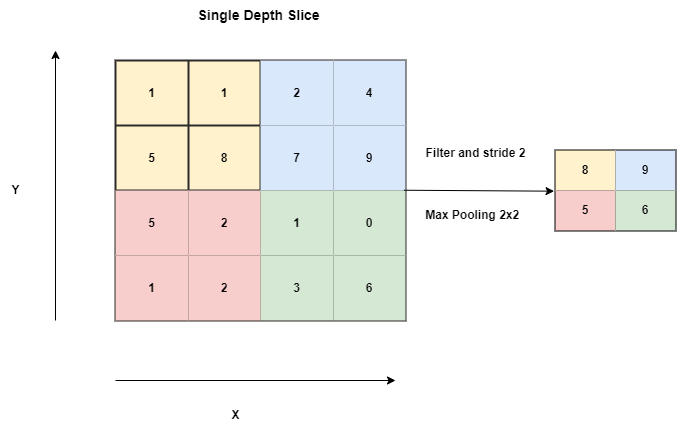
The pooling layer replaces the output of the network at certain locations by deriving a sum statistic of the nearby outputs.
This aids in reducing the spatial size of the representation, which declines the required amount of computation and weights. Each slice of the representation is subjected to the pooling operation separately.
There are several pooling functions such as the average of the rectangular neighborhood, L2 norm of the rectangular neighborhood, and a weighted average calculated using the distance from the central pixel.
Nevertheless, the most common process is max pooling, displaying the maximum output from the neighborhood.

Figure 4: Pooling Operation.
If there is an activation map of size W x W x D, a pooling kernel of spatial size F, and stride S, then the size of output volume can be determined by the following formula for padding layer:

Fully Connected Layer: Neurons in this layer have full connectivity with all neurons in the preceding and succeeding layer as seen in regular FCNN. This is why it can be computed as usual by a matrix multiplication followed by a bias effect.
The FC layer helps to map the representation between the input and the output.
1.3.4 Non-Linearity Layers:
There are several types of non-linear operations, the popular ones being:
Sigmoid: The sigmoid non-linearity has the mathematical form σ(κ) = 1/(1+e¯κ). It takes a real-valued number and represent it into a range between 0 and 1.
One notable drawback of the sigmoid activation function is its tendency to produce gradients close to zero when the activation values are located at the extreme ends of the function. This phenomenon poses a significant challenge during backpropagation, as the nearly-zero local gradient effectively hampers the flow of gradients, leading to the suppression of gradient information and hindering effective weight updates.
Another issue arises when the input data to the neuron is consistently positive, causing the sigmoid function to yield either all positive or all negative outputs. This, in turn, results in an oscillating pattern in the dynamics of gradient updates for the associated weights. Such oscillatory gradient behavior can adversely affect the convergence and stability of the learning process, compromising its effectiveness.
Tanh: Tanh squashes a real-valued number to the range [-1, 1]. Like sigmoid, the activation saturates, but — unlike the sigmoid neurons — its output is zero centered.
ReLU: The Rectified Linear Unit (ReLU) has become very popular in the last few years. It computes the function ƒ(κ)=max (0,κ). In other words, the activation is simply threshold at zero.
In comparison to sigmoid and tanh, ReLU is more reliable and accelerates the convergence by six times.
CNNs frequently consist of pooling layers, activation layers, and fully connected layers in addition to convolutional layers. While activation layers add non-linearity to the model by using an activation function like ReLU or sigmoid, pooling layers reduce the size of the feature maps by summing sets of neighboring data. In order to generate a forecast based on the learnt characteristics, fully linked layers are often utilized at the conclusion of the model.
To choose the best architecture for an assignment, scientists often experiment using various CNN designs while evaluating their performance on a validation set. Some factors that may influence the choice of architecture involve the size and complexity of the data being input, the available computational resources, and the desired level of precision.