Файл: В. И. Ульянова (Ленина) (СПбгэту лэти) Направление 27. 04. 04 Управление в технических системах Магистерская программа.docx

Another technique for hyperparameter optimization is random search. According to this method, a random sample of hyperparameters is taken from a predetermined range, and the network is trained using each set of hyperparameters. Grid search is more computationally expensive than random search, however random search may not necessarily produce the best hyperparameters.

Automated methods for hyperparameter optimization, like Bayesian optimization and evolutionary algorithms, have grown in favor recently. A probabilistic method called Bayesian optimization makes use of the past to direct the search for the ideal hyperparameters. Natural selection and genetics serve as the foundation for the search heuristic known as genetic algorithms. These methods may effectively search the hyperparameter space and identify the network's ideal hyperparameters.

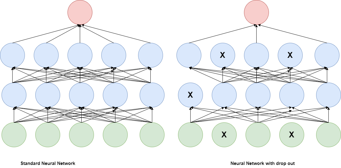
There are various methods for enhancing the performance of deep learning networks besides hyperparameter tweaking. Regularization is one such method that prevents overfitting by including a penalty term in the training loss function. L1 and L2 regularization, dropout, and early halting are all common regularization strategies.

Figure 9: The functionality of drop out.
Transfer learning is an additional method for enhancing the performance of deep learning networks. Transfer learning is the process of training a model on a new dataset using a previously trained model, often on a big dataset. This can enhance the performance of the network and considerably reduce the amount of data needed for training.

Improving deep learning networks is an essential aspect of achieving good performance and preventing overfitting. Hyperparameter optimization is a key technique for improving the performance of the network, and several techniques such as grid search, random search, Bayesian optimization, and genetic algorithms can be used for this purpose. Regularization techniques and transfer learning are also effective ways to improve the performance of deep learning networks.

3.1 Structure of Deep Learning:

Deep learning initiatives are intricate and need careful organization and preparation to be successful. A typical deep learning project goes through various steps, such as data collection and preparation, model selection and architecture design, model training and evaluation, and deployment.

The first stage in any deep learning project is data collection and preparation. Finding the data required for the project and obtaining it from multiple sources fall under this category. After the data has been gathered, it needs to be cleaned, preprocessed, and put into a form that the deep learning model can use. To expand the dataset, this may entail activities like feature extraction, data augmentation, and data normalization.

Model selection and architecture design make up the second stage. This entails creating the model's architecture and choosing the best deep learning algorithm for the given task. Convolutional neural networks (CNNs), recurrent neural networks (RNNs), and generative adversarial networks are a few of the deep learning techniques available. (GANs). The project's characteristics, such as the type of input data, the difficulty of the task, and the available computational resources, will determine the model's architecture.

The evaluation and training of models is the third stage. This requires using the preprocessed data to train the model and appropriate metrics to assess its success. Typically, a training set of data is used to train the model and a different validation set to validate it. To achieve the best performance, the model's hyperparameters, including the learning rate and regularization strength, must be fine-tuned. Using methods like transfer learning or ensemble learning, the model may also be refined.

The deployment phase is the last. In order to use the trained model to make predictions on fresh data, it must be integrated into a production environment. The model may then be integrated into an existing system or a web application, depending on the situation. In a production setting, it's critical to make sure the model is accurate, scalable, and efficient.

Deep learning initiatives should take an organized strategy in order to manage these stages efficiently. This entails segmenting the project into smaller jobs and establishing precise goals and deadlines for each work. Additionally, it's critical to keep thorough records of the project's data sources, preprocessing procedures, model architecture, and training information. This makes it easier to ensure that the project can be replicated and readily altered or expanded in the future.

When working on deep learning projects, there are other recommended practices that should be followed in addition to these stages. These include of employing cloud computing resources to scale out the training process, using version control to track changes to the code and data, and including explainability and interpretability in the model to boost openness and confidence.

3.2 Natural Language Processing using Voice Data:

Natural Language Processing (NLP) is a subfield of artificial intelligence that deals with the interaction between computers and human languages. Voice data, which entails collecting and processing speech signals to extract meaning and insights from spoken language, is a crucial component of NLP. Deep learning methods have attracted increasing attention in recent years as a way to enhance the precision and effectiveness of NLP tasks that use voice data.

Speech recognition, which involves translating spoken language into text, is one of the most popular NLP tasks employing voice data. Convolutional and recurrent neural networks (RNNs) and other deep learning models have been successfully used for this job, producing cutting-edge results on benchmark datasets like the Switchboard and LibriSpeech corpora. In order to anticipate the most likely transcription, these models first map speech signals to collections of phonemes or words.

Another important NLP task using voice data is speaker identification, which involves recognizing the identity of the person speaking. This is useful in applications such as security systems and call center routing. Deep learning models such as deep neural networks (DNNs) and support vector machines (SVMs) have been applied to this task, achieving high accuracy rates. These models work by extracting features from the speech signal, such as the pitch and frequency of the speaker's voice, and then using these features to classify the speaker.

Another area of research in NLP using voice data is sentiment analysis, which involves determining the emotional tone of a spoken sentence or passage. This is helpful in applications like social media monitoring and consumer feedback analysis. When applied to this problem, deep learning models like RNNs and CNNs have shown cutting-edge results on benchmark datasets like the SemEval Sentiment Analysis problem. These models learn to categorize speech signals based on additional characteristics including intonation and pace as well as the emotional content of the spoken words.

Several additional NLP applications, such as speech synthesis (which turns text into speech) and natural language comprehension, also employ voice data in addition to these tasks. (Analyzing the meaning of spoken language). In industries like assistive technology, education, and entertainment, these applications are crucial.

The unpredictability of speech signals, which can differ significantly based on parameters including the speaker's accent, background noise, and speech style, is a hurdle in NLP employing voice data. By learning to extract reliable features from the voice signal and reacting to changes in the input data, deep learning models can aid in solving this problem. The requirement for substantial amounts of labeled data for deep learning model training presents another difficulty. To be used for this, however, are a number of publicly accessible datasets, including the Common Voice corpus.

In general, NLP using voice data is a fast-expanding discipline with a wide range of applications and research potential. The accuracy and effectiveness of NLP tasks utilizing voice data have showed significant promise when using deep learning approaches, and it is expected that these techniques will continue to develop and advance in the years to come.
Conclusions:
In this chapter, the process of improving the performance of neural networks is discussed alongside some of the most important functions and methods that helps improve the implementation effectiveness of data and the increasing the accuracy of output.

4. VOICE PRE-PROCESSING USING DEEP LEARNING

4.1 Voice pre-processing:

Voice pre-processing is a crucial stage in deep learning voice cloning. In order to improve the quality of the voice data and lower any unwelcome noise or variability that could impair the neural network's accuracy, the audio recordings must be prepared for use in training.

There are several techniques used in voice pre-processing for voice cloning:

Noise reduction: Background noise from the recording area, electrical interference, or microphone hiss are all common issues with audio recordings. The audio recordings may be subjected to filters, such as a band-pass filter or a noise gate, to lessen noise. These filters assist in reducing unnecessary noise while keeping the essential elements of the voice.
Volume normalization: In order to bring the volume of various recordings closer to a uniform amplitude, normalizing involves adjusting the volume level. This can be accomplished by employing strategies like peak amplitude normalization or root-mean-square normalizing. The neural network is trained on constant volume levels across many recordings thanks to normalization.
Segmentation: Audio recordings are often long and continuous, and may contain multiple voices or different speaking styles. By breaking up the recordings into smaller units or segments, the neural network will be able to concentrate on particular traits and patterns in the target voice. Time intervals, phoneme or word boundaries, or speaker turns can all be used for segmentation. By giving the neural network the opportunity to concentrate on particular areas of the recording, segmentation can also aid to increase training efficiency.
Filtering: Low-pass and high-pass filters, among other methods, can be used to remove high-frequency noise or distortion from audio recordings. These filters assist in reducing unnecessary noise while keeping the essential elements of the voice.
Feature extraction: Extracting relevant features from the audio recordings can help the neural network to identify patterns and characteristics of the target voice. Pitch, formants, and spectral parameters like Mel frequency cepstral coefficients (MFCCs) are frequently employed in voice cloning. By giving the neural network more accurate information about the voice, feature extraction can increase its accuracy.

Voice pre-processing is a critical step in voice cloning using deep learning, as it helps to improve the quality and consistency of the voice data, and reduces the variability that could affect the accuracy of the neural network. Researchers can guarantee that the neural network is trained on high-quality sound data that accurately represents the target voice by using techniques including noise reduction, volume normalization, segmentation, filtering, and feature extraction.

4.2 Voice preprocessing implementation and logic:

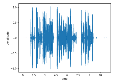
Sound Waves: A sound wave is a form of energy propagation that moves through a substance or material, known as a medium. It causes disturbances that can impact the positions and arrangements of particles within the initially balanced medium. The medium serves as a carrier for the wave, enabling its transmission from one location to another. Various substances like water, air, steel, and others can function as the medium for sound waves.

Figure 10: regular wave form.
When utilizing sound as raw data, there are significant challenges that arise. One crucial challenge is handling the high density of large samples, averaging around forty thousand samples per second of sound. Additionally, capturing long-range dependencies and effectively leveraging deep learning concepts and applications becomes challenging when dealing with extensive data sets. This includes addressing issues such as exclusion and feedback in convolutional networks and extending points for improved performance.

Therefore, a number of mathematical operations are implemented to improve signal processing

4.3 Fast Fourier Transform (FFT):

The Fast Fourier Transform (FFT) is a mathematical technique that converts a time-based function into its frequency-based counterpart. It enables the transformation from the time domain to the frequency domain. The FFT is an advancement of the Discrete Fourier Transform (DFT) that eliminates redundant calculations in the algorithm, resulting in a reduction in the number of mathematical operations required.

This optimization allows for the processing of large sample sizes without sacrificing the speed of the transformation. In fact, the FFT reduces the computational complexity by a factor of N/(log2(N)). Let x0, ...., xN-1 be complex numbers. Where DFT is defined by the formula:

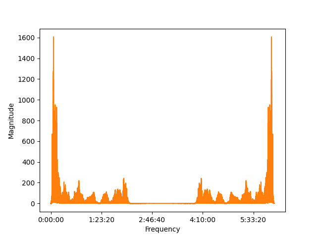
The output of the converted spectrum has the same number of sampling points, but half the values are redundant and are not usually shown in the spectrum, so the really useful information is N/2 + 1 point

Considering the original calculation complexity of the Discrete Fourier Transform (DFT) as N * N operations (where N represents the number of input sampling points), the Fast Fourier Transform (FFT) reduces this complexity to N * log10(N). For example, when calculating 1000 sampling points using the FFT algorithm, only 3000 calculations are needed, whereas the traditional DFT algorithm would require 1,000,000 calculations.

Figure 11: Frequency resolution and sampling time (inverse relationship).
By employing the FFT, the digital signal obtained from an oscilloscope can be efficiently converted.

After applying the FFT to N sampling points, the results of the FFT can be obtained for those N points. To facilitate the FFT process, it is common to choose N as a power of 2, ensuring compatibility with the algorithm.

Suppose the sampling frequency is Fs, the signal frequency is F, and the number of sampling points is N. Then the result after the FFT is a complex number with N points. Each point corresponds to a frequency point. The modulus at this point is the characteristic of the amplitude at this frequency

The frequency represented by a specific point, denoted as n, can be calculated using the formula: Fn = (n-1) * Fs/N. From the above formula, it is evident that the frequency resolved by Fn is Fs/N.

For instance, if the sampling frequency (Fs) is 1024 Hz and the number of sampling points (N) is also 1024, the resolution achieved is 1 Hz. In other words, when sampling at a rate of 1024 Hz for a duration of 1 second (which corresponds to 1024 points), performing an FFT allows for frequency analysis accurate to 1 Hz. If the signal is sampled for 2 seconds and subjected to FFT, the analysis can be accurate to 0.5 Hz. To enhance frequency accuracy, it is necessary to increase the number of sampling points, i.e., the sampling time.
Practical implementation:
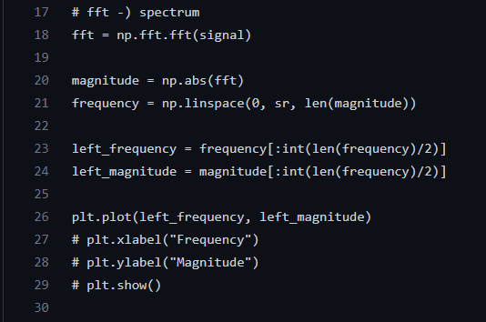
The fast Fourier transform is implemented in PyCharm python with the following code: