Файл: В. И. Ульянова (Ленина) (СПбгэту лэти) Направление 27. 04. 04 Управление в технических системах Магистерская программа.docx
ВУЗ: Не указан
Категория: Не указан
Дисциплина: Не указана
Добавлен: 25.10.2023
Просмотров: 299
Скачиваний: 1
СОДЕРЖАНИЕ
1.1 Explaining neural network:
1.2 Explaining the functionality of Neural Networks Works:
1.3.1 Convolutional Neural networks (CNN):
2. DESIGNING A CONVOLUTIONAL NEURAL NETWORK
2.1 Recurrent neural networks (RNNs):
2.2 Understanding Long Short-Term Memory (LSTM):
2.3 Describing LSTM mathematically:
2.4 Recurrent neural networks functionality in voice cloning applications:
3. IMPROVING DEEP LEARNING NETWORKS
3.1 Structure of Deep Learning:
3.2 Natural Language Processing using Voice Data:
4. VOICE PRE-PROCESSING USING DEEP LEARNING
4.2 Voice preprocessing implementation and logic:
4.3 Fast Fourier Transform (FFT):
4.4 Short-Time Fourier-Transform (STFT):
4.5 Mel frequency spectrum (MFCC):
4.7.3 Budling the autoencoder:
4.7.5 Results of the training process:
5.1 Explaining text to speech models (TTS):
5.2 DALL-E and its functionality:
5.3 Denoising Diffusion Probabilistic Models (DDPMs) and its functionality:
5.6 Implementing Tortoise-TTS:
5.6.2 Fine-Tuning Tortoise-TTS Model:
5.6.4 Installing Tortoise-TTS:
6.1 Compartment and validation of voice cloning output data:
7.2 Object and Company Description:
7.3 Market Analysis (Russia, Saint Petersburg):
7.4 Market Size and Growth Potential:
7.7 Marketing and Distribution Channels:
7.8 Regulatory and Cultural Considerations:
7.10 Economic Result Estimation:
7.11 Financial and Funding Plan:
4.4 Short-Time Fourier-Transform (STFT):
The overall result of FFT arithmetic can be significantly affected in the following scenarios: when the N sampling points lack a periodic pattern within the N-point FFT, when the signal is not a periodic function, or when a portion of the data is identified as noise. Utilizing FFT arithmetic under these circumstances can have a considerable impact on the final outcome.

where Z (t) is the source signal and g (t) is the port function and in order to facilitate computer processing, the signal is generally specified, and the specific formula is:

In practical terms, computing Short-Time Fourier Transforms (STFTs) involves dividing a longer time-based signal into segments of equal length and independently applying the Fourier transform to each segment. This process is akin to the FFT formula and involves the use of a Hamming window to ensure continuity and smoothness in the analysis.

Figure 14: types of windows
When utilizing the FFT to examine the frequency characteristics of a signal, the analysis is conducted on a finite set of data. The FFT treats a waveform as a discrete set of data points, whereas a continuous waveform consists of numerous small waveforms. In the context of the FFT, both the time and frequency domains are considered to be cyclic topologies. In the time domain, the waveform is assumed to be connected at its endpoints. These assumptions hold reasonably well if the measured signal is periodic and encompasses an integer number of periods at the time of acquisition.
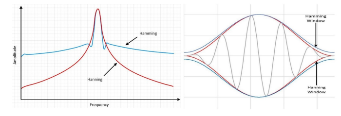
Figure 15: Hamming and Hanning windows
If the signal contains incorrect intervals, frequency leakage will occur. This can be improved by windowing.
The bounds of the finite sequence collected by the digitizer can be disconnected. Windowing reduces the size of these interruptions.
Practical implementation:
The Short Time Fourier transform is implemented in PyCharm python with the following code:
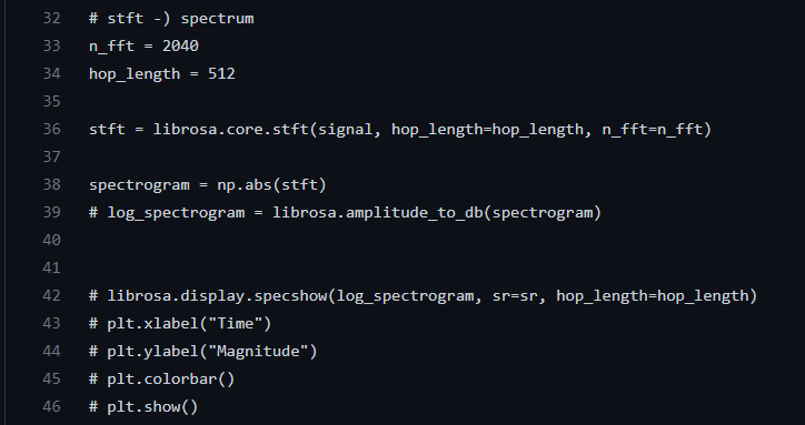
Figure 16: the code written to implement STFT on the voice sample
The result is changing as changing the (hop) parameter:
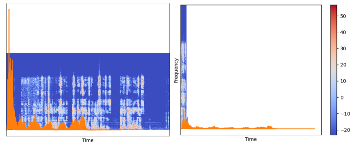
Figure 17: STFT with log (hop. l=16, right), and (hop. l = 512, left)
The (hop_length) values have been changed several times to monitor changes to the figure.
4.5 Mel frequency spectrum (MFCC):
The Mel-frequency cepstrum (MFC) is a method of representing the short-term power spectrum of a sound. It involves applying a linear cosine transform to the logarithm of the power spectrum, which is measured on a nonlinear Mel scale of frequency. This approach is commonly used in sound processing.
The Mel scale is a perceptual scale that captures the way listeners perceive pitches to be equally spaced from each other. It establishes a reference point by assigning a perceptual pitch of 1000 mels to a 1000 Hz tone, which is 40 dB above the listener's threshold. The Mel scale differs from the standard frequency measurement, and it is utilized as the basis for mapping frequencies in the MFC representation.
Above about 500 Hz, increasingly large intervals are judged by listeners to produce equal pitch increments.

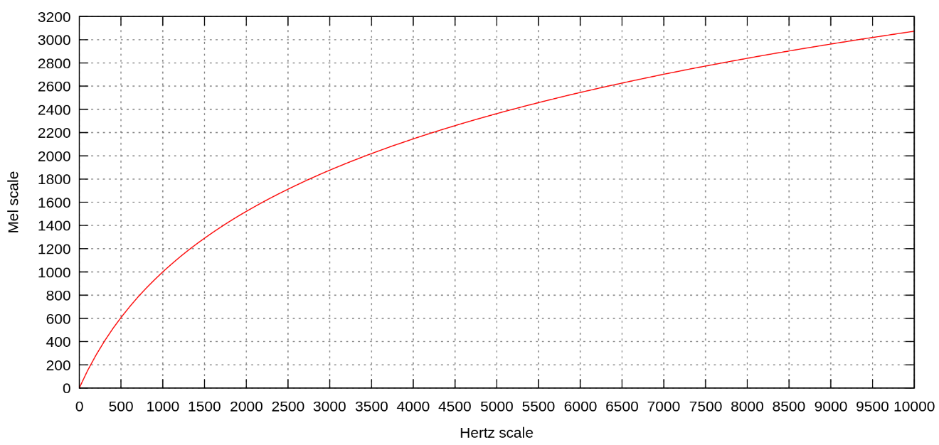
Figure 17: Mel spectrum graph.
MFCCs are commonly derived as follows:
The process involves applying the Fourier transform to extract frames of data, followed by mapping the obtained spectrum powers onto a slope scale using either triangular overlapping windows or cosine overlapping windows.
Subsequently, the magnitudes at each of the slope frequencies are recorded. Then, the discrete cosine transformation is applied to the list of logarithmic powers as if it were a signal.
The triangular window is defined as follows:
where N represents the length of the filter, and k ranges from 0 to N-1.
Different definitions may utilize N/2 or (N+1)/2 in the denominator of the last expression. This window is also known as the Bartlett window or the triangular window with zero endpoints when (N-1)/2 is used, as illustrated in the calculation above.
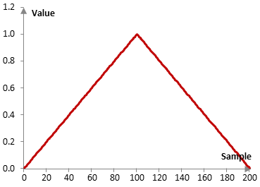
Figure 18: Triangular window.
Considering an N=201 low pass filter with a finite impulse response (FIR). The triangle window is shown below. Defining some important terms:
-
Window length is the length of the fixed intervals in which STFT divides the signal. -
Hop length is the length of the non-intersecting portion of window length. -
Overlap length is the length of the intersecting portion of the window length.
Static MFCC features, also known as cepstral coefficients, capture information from individual frames, providing a snapshot of the signal at a particular moment. To incorporate temporal dynamics, the first and second derivatives of the cepstral coefficients are computed. These derivatives are commonly referred to as delta coefficients (first-order derivative) and delta-delta coefficients (second-order derivative).
Delta coefficients reflect the speech pace, offering insights into the changes between consecutive frames. On the other hand, delta-delta coefficients indicate the speech acceleration, providing information about the rate of change in the speech signal.
The computation of dynamic parameters using the following method is widely adopted:
Compute the cepstral coefficients (static features) for each frame.
Compute the delta coefficients by taking the first-order derivative of the cepstral coefficients.
Compute the delta-delta coefficients by taking the second-order derivative of the cepstral coefficients.
By incorporating these dynamic parameters, a more comprehensive understanding of the temporal dynamics of the speech signal can be achieved.
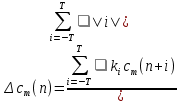 (20)
(20)where
 denotes the
  feature for the
  time frame,
  is the
  weight, and
  is the number of successive frames used for computation. Generally,
  is taken as 2. The delta-delta coefficients are computed by taking the first-order derivative of the delta coefficients.
Practical implementation:
The Mel-frequency spectrum (MFCC)is implemented in PyCharm python with the following code:
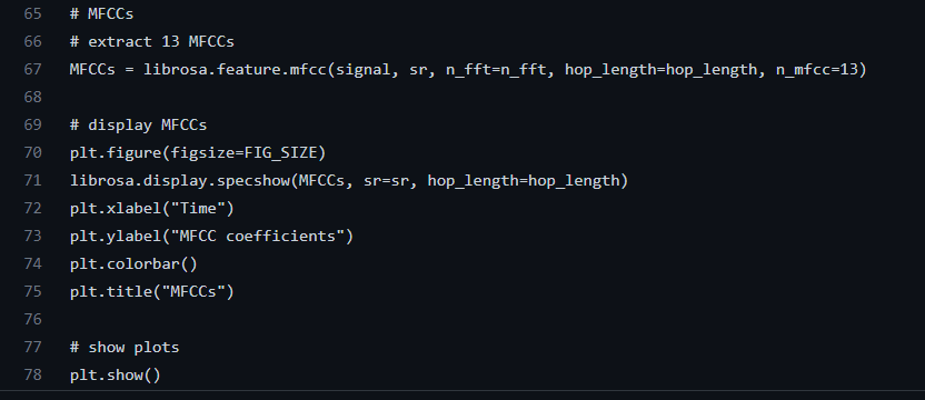
Figure 19: the code written to implement MFCC on the voice sample.
And the results as shown as following:
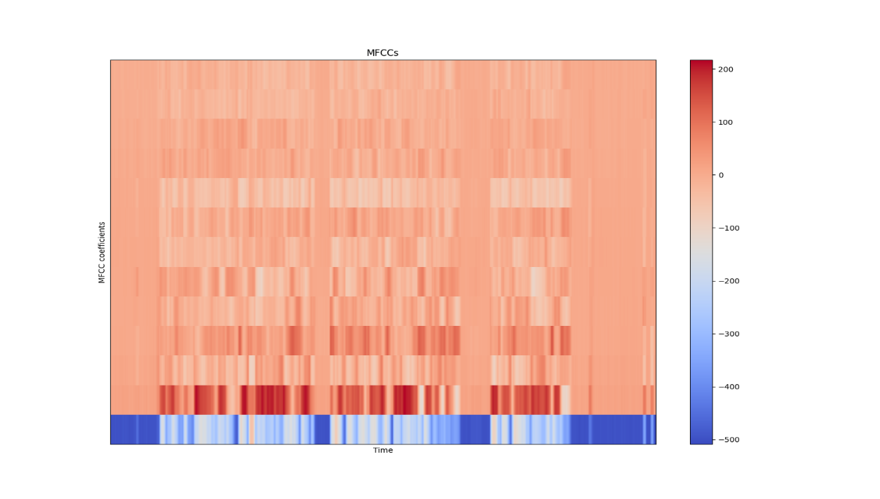
Figure 20: MFCC with color bar in (dB).
4.6 Using deferent library:
The final implementation using [NumPy, SciPy, zaf, matplotlib] which give us a more accurate representation of the (Mel-frequency spectrum) with the following code:
This Python module implements a number of functions for audio signal analysis.
Functions of zaf library:
-
[Stft] - Compute the short-time Fourier transform (STFT). -
[Istft] - Compute the inverse STFT. -
[Melfilterbank] - Compute the mel filterbank. -
[Mfcc] - Compute the mel-frequency cepstral coefficients (MFCCs) using a Mel filter bank. -
[Cqtkernel] - Compute the constant-Q transform (CQT) kernel. -
[cqtspectrogram] - Compute the CQT spectrogram using a CQT kernel. -
[Cqtchromagram] - Compute the CQT chromogram using a CQT kernel. -
[Dct] - Compute the discrete cosine transform (DCT) using the fast Fourier transform (FFT). -
[Dst] - Compute the discrete sine transform (DST) using the FFT. -
[Mdct] - Compute the modified discrete cosine transform (MDCT) using the FFT. -
[imdct] - Compute the inverse MDCT using the FFT.


Figure 21: the code written to implement MFCC using NumPy, SciPy.
# Import the needed modules
import numpy as np
import scipy.signal
import zaf
import matplotlib.pyplot as plt
# Read the audio signal (normalized) with its sampling frequency in Hz, and average it over its channels
audio_signal, sampling_frequency = zaf.wavread("Ali3.wav")
audio_signal = np.mean(audio_signal, 1)
# Set the parameters for the Fourier analysis
window_length = pow(2, int(np.ceil(np.log2(0.04*sampling_frequency))))
window_function = scipy.signal.hamming(window_length, sym=False)
step_length = int(window_length/2)
# Compute the mel filterbank
number_mels = 40
mel_filterbank = zaf.melfilterbank(sampling_frequency, window_length, number_mels)
# Compute the MFCCs using the filterbank
number_coefficients = 20
audio_mfcc = zaf.mfcc(audio_signal, window_function, step_length, mel_filterbank, number_coefficients)
# Compute the delta and delta-delta MFCCs
audio_dmfcc = np.diff(audio_mfcc, n=1, axis=1)
audio_ddmfcc = np.diff(audio_dmfcc, n=1, axis=1)
# Display the MFCCs, delta MFCCs, and delta-delta MFCCs in seconds
number_samples = len(audio_signal)
xtick_step = 1
plt.figure(figsize=(14, 7))
plt.subplot(3, 1, 1)
zaf.mfccshow(audio_mfcc, number_samples, sampling_frequency, xtick_step), plt.title("MFCCs")
plt.subplot(3, 1, 2)
zaf.mfccshow(audio_dmfcc, number_samples, sampling_frequency, xtick_step), plt.title("Delta MFCCs")
plt.subplot(3, 1, 3)
zaf.mfccshow(audio_ddmfcc, number_samples, sampling_frequency, xtick_step), plt.title("Delta-delta MFCCs")
plt.tight_layout()
plt.show()
The result is as the following figure shows:
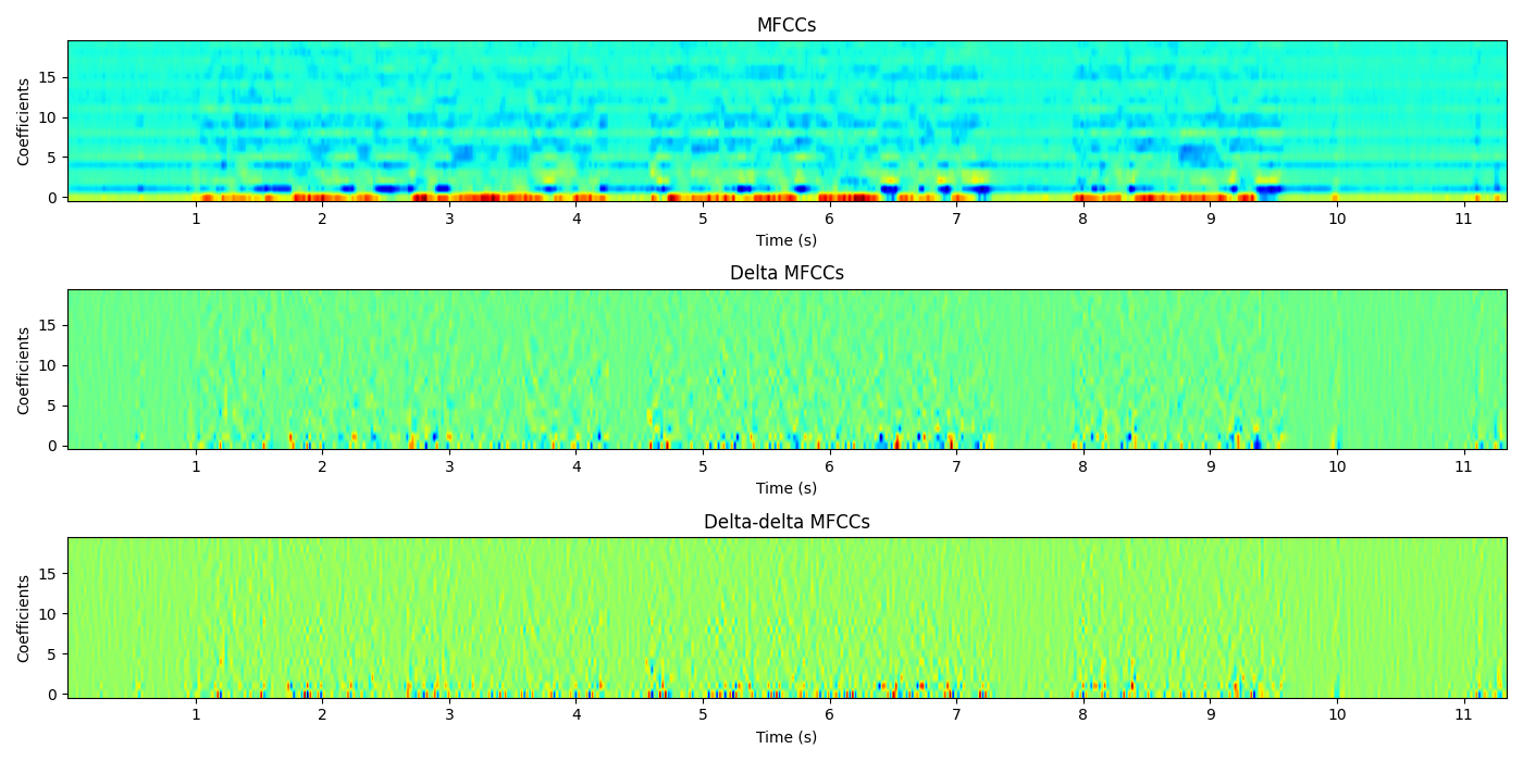

Figure 22: spectrum resulted from voice processing operation.
It is possible to simplify such complicated process by discussing the logic of (encoder-decoder).
4.7 Building the autoencoder:
The second part of approaching building a model capable of reproducing sound is to build an autoencoder capable of reading the image that produces the sound in the form of a spectrum, dismantling this image, extracting the features in it, and then re-installing it so that in the later stage can build a similar magnetic spectrum by simply giving it a spectrum Magnetic as input, resulting in a completely new output spectrum.
This process requires the construction of three parts, which are, respectively:
-
Encoder -
Decoder -
Autoencoder
The training data set is going to be MNIST for now as different results will be experienced with changing some of the parameters.