ВУЗ: Не указан
Категория: Не указан
Дисциплина: Не указана
Добавлен: 17.04.2021
Просмотров: 3757
Скачиваний: 3

Introduction to Python for Science, Release 0.9.23
t, N, dN
=
np
.
loadtxt(
"betaDecay.txt"
, skiprows
=
2
, unpack
=
True
)
########## Code to tranform & fit data starts here ##########
# Transform data and parameters to linear form: Y = A + B*X
X
=
t
# transform t data for fitting (trivial)
Y
=
np
.
log(N)
# transform N data for fitting
dY
=
dN
/
N
# transform uncertainties for fitting
# Fit transformed data X, Y, dY to obtain fitting parameters A & B
# Also returns uncertainties in A and B
B, A, dB, dA
=
LineFitWt(X, Y, dY)
# Return reduced chi-squared
redchisqr
=
redchisq(X, Y, dY, B, A)
# Determine fitting parameters for original exponential function
# N = N0 exp(-t/tau) ...
N0
=
np
.
exp(A)
tau
= -
1.0
/
B
# ... and their uncertainties
dN0
=
N0
*
dA
dtau
=
tau
**
2
*
dB
####### Code to plot transformed data and fit starts here #######
# Create line corresponding to fit using fitting parameters
# Only two points are needed to specify a straight line
Xext
=
0.05
*
(X
.
max()
-
X
.
min())
Xfit
=
np
.
array([X
.
min()
-
Xext, X
.
max()
+
Xext])
Yfit
=
A
+
B
*
Xfit
plt
.
errorbar(X, Y, dY, fmt
=
"bo"
)
plt
.
plot(Xfit, Yfit,
"r-"
, zorder
=-
1
)
plt
.
xlim(
0
,
100
)
plt
.
ylim(
1.5
,
7
)
plt
.
title(
"$\mathrm{Fit
\\
to:}
\\
\ln N = -t/
\\
tau + \ln N_0$"
)
plt
.
xlabel(
"t"
)
plt
.
ylabel(
"ln(N)"
)
plt
.
text(
50
,
6.6
,
"A = ln N0 = {0:0.2f} $\pm$ {1:0.2f}"
.
format(A, dA))
plt
.
text(
50
,
6.3
,
"B = -1/tau = {0:0.4f} $\pm$ {1:0.4f}"
.
format(
-
B, dB))
plt
.
text(
50
,
6.0
,
"$\chi_r^2$ = {0:0.3f}"
.
format(redchisqr))
8.1. Using linear regression for fitting non-linear functions
145

Introduction to Python for Science, Release 0.9.23
plt
.
text(
50
,
5.7
,
"N0 = {0:0.0f} $\pm$ {1:0.0f}"
.
format(N0, dN0))
plt
.
text(
50
,
5.4
,
"tau = {0:0.1f} $\pm$ {1:0.1f} days"
.
format(tau, dtau))
plt
.
show()
8.1.2 Linear regression for fitting a power-law function
You can use a similar approach to the one outlined above to fit experimental data to a
power law fitting function of the form
P
(
s
) =
P
0
s
α
.
(8.7)
We follow the same approach we used for the exponential fitting function and first take
the logarithm of both sides of (
ln
P
= ln
P
0
+
α
ln
s .
(8.8)
We recast this in the form of a linear equation
y
=
a
+
bx
with the following identifica-
tions:
x
= ln
s
y
= ln
P
a
= ln
P
0
b
=
α
(8.9)
Following a procedure similar to that used to fit using an exponential fitting function, you
can use the tranformations given by (
) as the basis for a program to fit a power-law
fitting function such as (
) to experimental data.
8.2 Nonlinear fitting
The method introduced in the previous section for fitting nonlinear fitting functions can
be used only if the fitting function can be transformed into a fitting function that is linear
in the fitting parameters
a
,
b
,
c
... When we have a nonlinear fitting function that cannot
be transformed into a linear form, we need another approach.
The problem of finding values of the fitting parameters that minimize
χ
2
is a nonlinear op-
timization problem to which there is quite generally no analytical solution (in contrast to
146
Chapter 8. Curve Fitting


Introduction to Python for Science, Release 0.9.23
the linear optimization problem). We can gain some insight into this nonlinear optimiza-
tion problem, namely the fitting of a nonlinear fitting function to a data set, by considering
a fitting function with only two fitting parameters. That is, we are trying to fit some data
set
{
x
i
, y
i
}
, with uncertainties in
{
y
i
}
of
{
σ
i
}
, to a fitting function is
f
(
x
;
a, b
)
where
a
and
b
are the two fitting parameters. To do so, we look for the minimum in
χ
2
(
a, b
) =
X
i
y
i
−
f
(
x
i
)
σ
i
2
.
Note that once the data set, uncertainties, and fitting function are specified,
χ
2
(
a, b
)
is
simply a function of
a
and
b
. We can picture the function
χ
2
(
a, b
)
as a of landscape with
peaks and valleys: as we vary
a
and
b
,
χ
2
(
a, b
)
rises and falls. The basic idea of all
nonlinear fitting routines is to start with some initial guesses for the fitting parameters,
here
a
and
b
, and by scanning the
χ
2
(
a, b
)
landscape, find values of
a
and
b
that minimize
χ
2
(
a, b
)
.
There are a number of different methods for trying to find the minimum in
χ
2
for non-
linear fitting problems. Nevertheless, the method that is most widely used goes by the
name of the
Levenberg-Marquardt
method. Actually the Levenberg-Marquardt method
is a combination of two other methods, the
steepest descent
(or gradient) method and
parabolic extrapolation
. Roughly speaking, when the values of
a
and
b
are not too near
their optimal values, the gradient descent method determines in which direction in
(
a, b
)
-
space the function
χ
2
(
a, b
)
decreases most quickly—the direction of steepest descent—
and then changes
a
and
b
accordingly to move in that direction. This method is very
efficient unless
a
and
b
are very near their optimal values. Near the optimal values of
a
and
b
, parabolic extrapolation is more efficient. Therefore, as
a
and
b
approach their
optimal values, the Levenberg-Marquardt method gradually changes to the parabolic ex-
trapolation method, which approximates
χ
2
(
a, b
)
by a Taylor series second order in
a
and
b
and then computes directly the analytical minimum of the Taylor series approximation
of
χ
2
(
a, b
)
. This method is only good if the second order Taylor series provides a good
approximation of
χ
2
(
a, b
)
. That is why parabolic extrapolation only works well very near
the minimum in
χ
2
(
a, b
)
.
Before illustrating the Levenberg-Marquardt method, we make one important cautionary
remark: the Levenberg-Marquardt method can fail if the initial guesses of the fitting pa-
rameters are too far away from the desired solution. This problem becomes more serious
the greater the number of fitting parameters. Thus it is important to provide reasonable
initial guesses for the fitting parameters. Usually, this is not a problem, as it is clear from
the physical situation of a particular experiment what reasonable values of the fitting pa-
rameters are. But beware!
The
scipy.optimize
module provides routines that implement the Levenberg-
Marquardt non-linear fitting method. One is called
scipy.optimize.leastsq
.
8.2. Nonlinear fitting
147

Introduction to Python for Science, Release 0.9.23
A
somewhat
more
user-friendly
version
of
the
same
method
is
accessed
through another routine in the same
scipy.optimize
module:
it’s called
scipy.optimize.curve_fit
and it is the one we demonstrate here.
The
function call is
import scipy.optimize
[... insert code here ...]
scipy.optimize.curve_fit(f, xdata, ydata, p0=None, sigma=None,
**kwargs)
The arguments of
curve_fit
are
•
f(xdata, a, b, ...)
: is the fitting function where
xdata
is the data for the
independent variable and
a, b, ...
are the fitting parameters, however many
there are, listed as separate arguments. Obviously,
f(xdata, a, b, ...)
should return the
y
value of the fitting function.
•
xdata
: is the array containing the
x
data.
•
ydata
: is the array containing the
y
data.
•
p0
: is a tuple containing the initial guesses for the fitting parameters. The guesses
for the fitting parameters are set equal to 1 if they are left unspecified. It is almost
always a good idea to specify the initial guesses for the fitting parameters.
•
sigma
: is the array containing the uncertainties in the
y
data.
•
**kwargs
: are keyword arguments that can be passed to the fitting routine
scipy.optimize.leastsq
that
curve_fit
calls. These are usually left
unspecified.
We demonstrate the use of
curve_fit
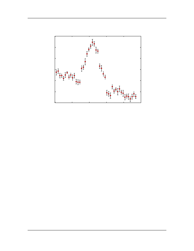
to fit the data plotted in the figure below:
We model the data with the fitting function that consists of a quadratic polynomial back-
ground with a Gaussian peak:
A
(
f
) =
a
+
bf
+
cf
2
+
P e
−
1
2
[(
f
−
f
p
)
/f
w
]
2
.
Lines 7 and 8 define the fitting functions. Note that the independent variable
f
is the first
argument, which is followed by the six fitting parameters
a
,
b
,
c
,
P
,
f
p
, and
f
w
.
To fit the data with
A
(
f
)
, we need good estimates of the fitting parameters. Setting
f
= 0
,
we see that
a
≈
60
. An estimate of the slope of the baseline gives
b
≈ −
60
/
20 =
−
3
.
The curvature in the baseline is small so we take
c
≈
0
. The amplitude of the peak above
the baseline is
P
≈
80
. The peak is centered at
f
p
≈
11
, while width of peak is about
f
w
≈
2
. We use these estimates to set the initial guesses of the fitting parameters in lines
14 and 15 in the code below.
148
Chapter 8. Curve Fitting
Introduction to Python for Science, Release 0.9.23
0
5
10
15
20
25
frequency (THz)
0
20
40
60
80
100
120
absorption (arb units)
The function that performs the Levenverg-Marquardt algorithm,
scipy.optimize.curve_fit
,
is called in lines 19-20 with the output set equal to the one and two-dimensional arrays
nlfit
and
nlpcov
, respectively. The array
nlfit
, which gives the optimal values of
the fitting parameters, is unpacked in line 23. The square root of the diagonal of the two-
dimensional array
nlpcov
, which gives the estimates of the uncertainties in the fitting
parameters, is unpacked in lines 26-27 using a list comprehension.
The rest of the code plots the data, the fitting function using the optimal values of the
fitting parameters found by
scipy.optimize.curve_fit
, and the values of the
fitting parameters and their uncertainties.
1
import
numpy
as
np
2
import
matplotlib.pyplot
as
plt
3
import
matplotlib.gridspec
as
gridspec
# for unequal plot boxes
4
import
scipy.optimize
5
6
# define fitting function
7
def
GaussPolyBase
(f, a, b, c, P, fp, fw):
8
return
a
+
b
*
f
+
c
*
f
*
f
+
P
*
np
.
exp(
-
0.5
*
((f
-
fp)
/
fw)
**
2
)
9
10
# read in spectrum from data file
11
# f=frequency, s=signal, ds=s uncertainty
12
f, s, ds
=
np
.
loadtxt(
"Spectrum.txt"
, skiprows
=
4
, unpack
=
True
)
13
8.2. Nonlinear fitting
149