ВУЗ: Не указан
Категория: Не указан
Дисциплина: Не указана
Добавлен: 17.04.2021
Просмотров: 3708
Скачиваний: 3

Introduction to Python for Science, Release 0.9.23
14
# initial guesses for fitting parameters
15
a0, b0, c0
=
60.
,
-
3.
,
0.
16
P0, fp0, fw0
=
80.
,
11.
,
2.
17
18
# fit data using SciPy’s Levenberg-Marquart method
19
nlfit, nlpcov
=
scipy
.
optimize
.
curve_fit(GaussPolyBase,
20
f, s, p0
=
[a0, b0, c0, P0, fp0, fw0], sigma
=
ds)
21
22
# unpack fitting parameters
23
a, b, c, P, fp, fw
=
nlfit
24
# unpack uncertainties in fitting parameters from diagonal
25
# of covariance matrix
26
da, db, dc, dP, dfp, dfw
=
\
27
[np
.
sqrt(nlpcov[j,j])
for
j
in
range
(nlfit
.
size)]
28
29
# create fitting function from fitted parameters
30
f_fit
=
np
.
linspace(
0.0
,
25.
,
128
)
31
s_fit
=
GaussPolyBase(f_fit, a, b, c, P, fp, fw)
32
33
# Calculate residuals and reduced chi squared
34
resids
=
s
-
GaussPolyBase(f, a, b, c, P, fp, fw)
35
redchisqr
=
((resids
/
ds)
**
2
)
.
sum()
/
float
(f
.
size
-
6
)
36
37
# Create figure window to plot data
38
fig
=
plt
.
figure(
1
, figsize
=
(
8
,
8
))
39
gs
=
gridspec
.
GridSpec(
2
,
1
, height_ratios
=
[
6
,
2
])
40
41
# Top plot: data and fit
42
ax1
=
fig
.
add_subplot(gs[
0
])
43
ax1
.
plot(f_fit, s_fit)
44
ax1
.
errorbar(f, s, yerr
=
ds, fmt
=
’or’
, ecolor
=
’black’
)
45
ax1
.
set_xlabel(
’frequency (THz)’
)
46
ax1
.
set_ylabel(
’absorption (arb units)’
)
47
ax1
.
text(
0.7
,
0.95
,
’a = {0:0.1f}$\pm${1:0.1f}’
48
.
format(a, da), transform
=
ax1
.
transAxes)
49
ax1
.
text(
0.7
,
0.90
,
’b = {0:0.2f}$\pm${1:0.2f}’
50
.
format(b, db), transform
=
ax1
.
transAxes)
51
ax1
.
text(
0.7
,
0.85
,
’c = {0:0.2f}$\pm${1:0.2f}’
52
.
format(c, dc), transform
=
ax1
.
transAxes)
53
ax1
.
text(
0.7
,
0.80
,
’P = {0:0.1f}$\pm${1:0.1f}’
54
.
format(P, dP), transform
=
ax1
.
transAxes)
55
ax1
.
text(
0.7
,
0.75
,
’fp = {0:0.1f}$\pm${1:0.1f}’
56
.
format(fp, dfp), transform
=
ax1
.
transAxes)
57
ax1
.
text(
0.7
,
0.70
,
’fw = {0:0.1f}$\pm${1:0.1f}’
58
.
format(fw, dfw), transform
=
ax1
.
transAxes)
150
Chapter 8. Curve Fitting

Introduction to Python for Science, Release 0.9.23
59
ax1
.
text(
0.7
,
0.60
,
’$\chi_r^2$ = {0:0.2f}’
60
.
format(redchisqr),transform
=
ax1
.
transAxes)
61
ax1
.
set_title(
’$s(f) = a+bf+cf^2+P\,e^{-(f-f_p)^2/2f_w^2}$’
)
62
63
# Bottom plot: residuals
64
ax2
=
fig
.
add_subplot(gs[
1
])
65
ax2
.
errorbar(f, resids, yerr
=
ds, ecolor
=
"black"
, fmt
=
"ro"
)
66
ax2
.
axhline(color
=
"gray"
, zorder
=-
1
)
67
ax2
.
set_xlabel(
’frequency (THz)’
)
68
ax2
.
set_ylabel(
’residuals’
)
69
ax2
.
set_ylim(
-
20
,
20
)
70
ax2
.
set_yticks((
-
20
,
0
,
20
))
71
72
plt
.
show()
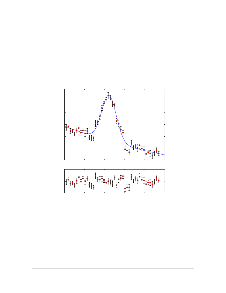
The above code also plots the difference between the data and fit, known as the
residuals
in the subplot below the plot of the data and fit. Plotting the residuals in this way gives
a graphical representation of the goodness of the fit. To the extent that the residuals vary
randomly about zero and do not show any overall upward or downward curvature, or any
long wavelength oscillations, the fit would seem to be a good fit.
Finally, we note that we have used the MatPlotLib package
gridspec
to create the two
subplots with different heights. The
gridspec
are made in lines 3 (where the package
is imported), 36 (where 2 rows and 1 column are specified with relative heights of 6 to 2),
39 (where the first
gs[0]
height is specified), and 54 (where the second
gs[1]
height
is specified). More details about the
gridspec
package can be found at the MatPlotLib
web site.
8.2. Nonlinear fitting
151

Introduction to Python for Science, Release 0.9.23
0
5
10
15
20
25
frequency (THz)
0
20
40
60
80
100
120
absorption (arb units)
a = 57.1
±
2.8
b = -2.55
±
0.80
c = 0.02
±
0.03
P = 77.5
±
3.5
fp = 11.1
±
0.1
fw = 1.8
±
0.1
χ
2
r
= 2.03
s
(
f
) =
a
+
bf
+
cf
2
+
P e
−
(
f
−
f
p
)
2
/
2
f
2
w
0
5
10
15
20
25
frequency (THz)
20
0
20
residuals
Figure 8.2: Fit to Gaussian with quadratic polynomial background.
152
Chapter 8. Curve Fitting

Introduction to Python for Science, Release 0.9.23
8.3 Exercises
1. When a voltage source is connected across a resistor and inductor in series, the
voltage across the inductor
V
i
(
t
)
is predicted to obey the equation
V
(
t
) =
V
0
e
−
Γ
t
(8.10)
where
t
is the time and the decay rate
Γ =
R/L
is the ratio of the resistance
R
to
the inductance
L
of the circuit. In this problem, you are to write a Python routine
that fits the above equation to the data below for the voltage measured across an
inductor after it is connected in series with a resistor to a voltage source. Following
the example in the text, linearize the (
) and use a linear fitting routine, either
the one you wrote from the previous chapter or one from NumPy or SciPy.
(a) Find the best values of
Γ
and
V
0
and the uncertainties in their values
σ
Γ
and
σ
V
0
.
(b) Find the value of
χ
2
r
for your fit. Does it make sense?
(c) Make a semi-log plot of the data using symbols with error bars (no line) and
of the fit (line only). The fit should appear as a straight line that goes through
the data points.
(d) If the resistor has a value of 10.0
kΩ
, what is the value of the inductance and
its uncertainty according to your fit, assuming that the error in the resistance
is negligibly small.
Data for decay of voltage across an inductor
in an RL circuit
Date: 24-Oct-2012
Data taken by D. M. Blantogg and T. P. Chaitor
time (ns)
voltage (volts)
uncertainty (volts)
0.0
5.08e+00
1.12e-01
32.8
3.29e+00
9.04e-02
65.6
2.23e+00
7.43e-02
98.4
1.48e+00
6.05e-02
131.2
1.11e+00
5.25e-02
164.0
6.44e-01
4.00e-02
196.8
4.76e-01
3.43e-02
229.6
2.73e-01
2.60e-02
262.4
1.88e-01
2.16e-02
295.2
1.41e-01
1.87e-02
328.0
9.42e-02
1.53e-02
360.8
7.68e-02
1.38e-02
8.3. Exercises
153

Introduction to Python for Science, Release 0.9.23
393.6
3.22e-02
8.94e-03
426.4
3.22e-02
8.94e-03
459.2
1.98e-02
7.01e-03
492.0
1.98e-02
7.01e-03
2. Small nanoparticles of soot suspended in water start to aggregate when salt is added.
The average radius
r
of the aggregates is predicted to grow as a power law in time
t
according to the equation
r
=
r
0
t
n
. Taking the logarithm of this equation gives
ln
r
=
n
ln
t
+ ln
r
0
. Thus the data should fall on a straight line if
ln
r
is plotted
vs
ln
t
.
(a) Plot the data below on a graph of
ln
r
vs
ln
t
to see if the data fall approxi-
mately on a straight line.
Size of growing aggregate
Date: 19-Nov-2013
Data taken by M. D. Gryart and M. L. Waites
time (m)
size (nm)
unc (nm)
0.12
115
10
0.18
130
12
0.42
202
14
0.90
335
18
2.10
510
20
6.00
890
30
18.00
1700
40
42.00
2600
50
(b) Defining
y
= ln
r
and
x
= ln
t
, use the linear fitting routine you wrote for the
previous problem to fit the data and find the optimal values for the slope and
y
intercept, as well as their uncertainties. Use these fitted values to find the
optimal values of the the amplitude
r
0
and the power
n
in the fitting function
r
=
r
0
t
n
. What are the fitted values of
r
0
and
n
? What is the value of
χ
2
r
?
Does a power law provide an adequate model for the data?
3. In this problem you explore using a non-linear least square fitting routine to fit the
data shown in the figure below. The data, including the uncertainties in the
y
values,
are provided in the table below. Your task is to fit the function
d
(
t
) =
A
(1 +
B
cos
ωt
)
e
−
t
2
/
2
τ
2
+
C
(8.11)
to the data, where the fitting parameters are
A
,
B
,
C
,
ω
, and
τ
.
(a) Write a Python program that (
i
) reads the data in from a data file, (
ii
) defines a
function
oscDecay(t, A, B, C, tau, omega)
for the function
d
(
t
)
above, and (
iii
) produces a plot of the data and the function
d
(
t
)
. Choose the
154
Chapter 8. Curve Fitting