ВУЗ: Не указан
Категория: Не указан
Дисциплина: Не указана
Добавлен: 17.04.2021
Просмотров: 3715
Скачиваний: 3
Introduction to Python for Science, Release 0.9.23
0
5
10
15
20
25
30
35
40
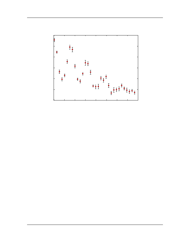
time (ms)
15
20
25
30
35
40
45
decay (arb units)
fitting parameters
A
,
B
,
C
,
tau
, and
omega
to produce an approximate fit
“by eye” to the data. You should be able estimate reasonable values for these
parameters just by looking at the data and thinking about the behavior of
d
(
t
)
.
For example,
d
(0) =
A
(1+
B
)+
C
while
d
(
∞
) =
C
. What parameter in
d
(
t
)
controls the period of the peaks observed in the data? Use that information to
estimate the value of that parameter.
(b) Following the example in section
, write a program using the
SciPy function
scipy.optimize.curve_fit
to fit Eq. (
) to the
data and thus find the optimal values of the fitting parameters
A
,
B
,
C
,
ω
,
and
τ
. Your program should plot the data along with the fitting function using
the optimal values of the fitting parameters. Write a function to calculate the
reduced
χ
2
. Print out the value of the reduced
χ
2
on your plot along with the
optimal values of the fitting parameters. You can use the results from part (a)
to estimate good starting values of the fitting parameters
(c) Once you have found the optimal fitting parameters, run your fitting program
again using for starting values the optimal values of the fitting parameters
A
,
B
,
C
, and
τ
, but set the starting value of
ω
to be 3 times the optimal value. You
should find that the program converges to a different set of fitting parameters
than the ones you found in part (b). Using the program you wrote for part (b)
make a plot of the data and the fit like the one you did for part (a). The fit
should be noticeably worse. What is the value of the reduced
χ
2
for this fit; it
8.3. Exercises
155

Introduction to Python for Science, Release 0.9.23
should be much larger than the one you found for part (c). The program has
found a local minimum in
χ
2
—one that is obviously is not the best fit!
(d) Setting the fitting parameters
A
,
B
,
C
, and
τ
to the optimal values you found
in part (b), plot
χ
2
r
as a function of
ω
for
ω
spanning the range from 0.05 to
3.95. You should observe several local minima for different values of
χ
2
r
; the
global minimum in
χ
2
r
should occur for the optimal value of
ω
you found in
part (b).
Data for absorption spectrum
Date: 21-Nov-2012
Data taken by P. Dubson and M. Sparks
time (ms)
signal
uncertainty
0.2
41.1
0.9
1.4
37.2
0.9
2.7
28.3
0.9
3.9
24.8
1.1
5.1
27.8
0.8
6.4
34.5
0.7
7.6
39.0
0.9
8.8
37.7
0.8
10.1
29.8
0.9
11.3
22.2
0.7
12.5
22.3
0.6
13.8
26.7
1.1
15.0
30.4
0.7
16.2
32.6
0.8
17.5
28.9
0.8
18.7
22.9
1.3
19.9
21.7
0.9
21.1
22.1
1.0
22.4
22.3
1.0
23.6
26.3
1.0
24.8
26.2
0.8
26.1
21.4
0.9
27.3
20.0
1.0
28.5
20.1
1.2
29.8
21.2
0.5
31.0
22.0
0.9
32.2
21.6
0.7
33.5
21.0
0.7
34.7
19.7
0.9
35.9
17.9
0.9
37.2
18.1
0.8
38.4
18.9
1.1
156
Chapter 8. Curve Fitting


CHAPTER
NINE
NUMERICAL ROUTINES:
SCIPY AND NUMPY
SciPy is a Python library of mathematical routines. Many of the SciPy routines are Python
“wrappers”, that is, Python routines that provide a Python interface, for numerical li-
braries and routines originally written in Fortran, C, or C++. Thus, SciPy lets you take
advantage of the decades of work that has gone into creating and optimizing numerical
routines for science and engineering. Because the Fortran, C, or C++ code that Python
accesses is compiled, these routines typically run very fast. Therefore, there is no real
downside—no speed penalty—for using Python in these cases.
We have already encountered one of SciPy’s routines,
scipy.optimize.leastsq
,
for fitting nonlinear functions to experimental data, which was introduced in the the chap-
ter on
. Here we will provide a further introduction to a number of other
SciPy packages, in particular those on special functions, linear algebra, finding roots of
scalar functions, discrete Fourier transforms, and numerical integration, including rou-
tines for numerically solving ordinary differential equations (ODEs). Our introduction to
these capabilities does not include extensive background on the numerical methods em-
ployed; that is a topic for another text. Here we simply introduce the SciPy routines for
performing some of the more frequently required numerical tasks.
One final note: SciPy makes extensive use of NumPy arrays, so NumPy should always be
imported with SciPy
157
Introduction to Python for Science, Release 0.9.23
9.1 Special functions
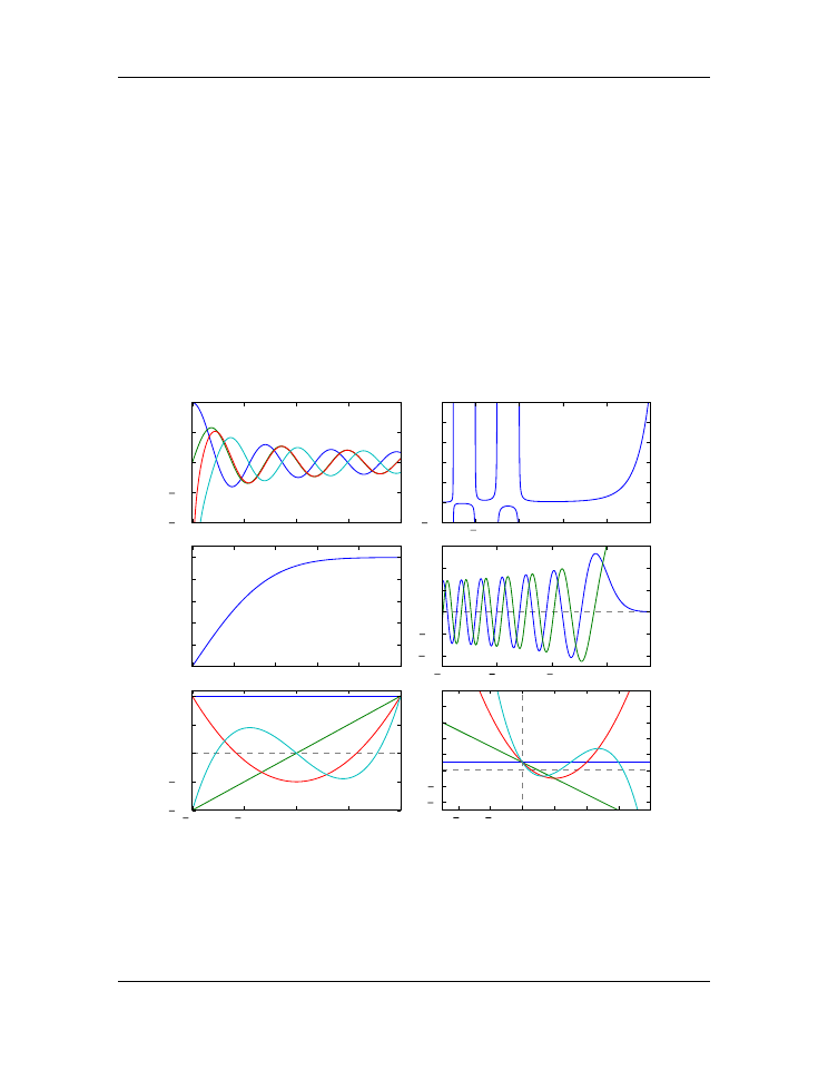
SciPy provides a plethora of special functions, including Bessel functions (and routines
for finding their zeros, derivatives, and integrals), error functions, the gamma function,
Legendre, Laguerre, and Hermite polynomials (and other polynomial functions), Mathieu
functions, many statistical functions, and a number of other functions. Most are contained
in the
scipi.special
library, and each has its own special arguments and syntax, de-
pending on the vagaries of the particular function. We demonstrate a number of them in
the code below that produces a plot of the different functions called. For more informa-
tion, you should consult the SciPy web site on the
scipy.special
library.
0
5
10
15
20
1.0
0.5
0.0
0.5
1.0
Bessel
2
0
2
4
6
20
0
20
40
60
80
100
Gamma
0.0
0.5
1.0
1.5
2.0
2.5
0.0
0.2
0.4
0.6
0.8
1.0
Error
15
10
5
0
0.4
0.2
0.0
0.2
0.4
Airy
1.0
0.5
0.0
0.5
1.0
1.0
0.5
0.0
0.5
1.0
Legendre
4
2
0
2
4
6
8
4
2
0
2
4
6
8
10
Laguerre
Figure 9.1: Plots of special functions
158
Chapter 9. Numerical Routines: SciPy and NumPy

Introduction to Python for Science, Release 0.9.23
1
import
numpy
as
np
2
import
scipy
as
sp
3
import
matplotlib.pyplot
as
plt
4
5
# create a figure window
6
fig
=
plt
.
figure(
1
, figsize
=
(
9
,
8
))
7
8
# create arrays for a few Bessel functions and plot them
9
x
=
np
.
linspace(
0
,
20
,
256
)
10
j0
=
sp
.
special
.
jn(
0
, x)
11
j1
=
sp
.
special
.
jn(
1
, x)
12
y0
=
sp
.
special
.
yn(
0
, x)
13
y1
=
sp
.
special
.
yn(
1
, x)
14
ax1
=
fig
.
add_subplot(
321
)
15
ax1
.
plot(x,j0, x,j1, x,y0, x,y1)
16
ax1
.
set_ylim(
-
1
,
1
)
17
ax1
.
text(
0.5
,
0.95
,
’Bessel’
, ha
=
’center’
, va
=
’top’
,
18
transform
=
ax1
.
transAxes)
19
20
# gamma function
21
x
=
np
.
linspace(
-
3.5
,
6.
,
3601
)
22
g
=
sp
.
special
.
gamma(x)
23
g
=
np
.
ma
.
masked_outside(g,
-
100
,
400
)
24
ax2
=
fig
.
add_subplot(
322
)
25
ax2
.
plot(x,g)
26
ax2
.
set_xlim(
-
3.5
,
6
)
27
ax2
.
set_ylim(
-
20
,
100
)
28
ax2
.
text(
0.5
,
0.95
,
’Gamma’
, ha
=
’center’
, va
=
’top’
,
29
transform
=
ax2
.
transAxes)
30
31
# error function
32
x
=
np
.
linspace(
0
,
2.5
,
256
)
33
ef
=
sp
.
special
.
erf(x)
34
ax3
=
fig
.
add_subplot(
323
)
35
ax3
.
plot(x,ef)
36
ax3
.
set_ylim(
0
,
1.1
)
37
ax3
.
text(
0.5
,
0.95
,
’Error’
, ha
=
’center’
, va
=
’top’
,
38
transform
=
ax3
.
transAxes)
39
40
# Airy function
41
x
=
np
.
linspace(
-
15
,
4
,
256
)
42
ai, aip, bi, bip
=
sp
.
special
.
airy(x)
43
ax4
=
fig
.
add_subplot(
324
)
44
ax4
.
plot(x,ai, x,bi)
9.1. Special functions
159