ВУЗ: Не указан
Категория: Не указан
Дисциплина: Не указана
Добавлен: 17.04.2021
Просмотров: 3716
Скачиваний: 3

Introduction to Python for Science, Release 0.9.23
Generalized eigenvalue problem
The
scipy.linalg.eig
function can also solve the
generalized
eigenvalue problem
A
x
=
λ
B
x
where
B
is a square matrix with the same size as
A
. Suppose, for example, that we have
In [22]:
A
=
array([[
2
,
4
,
6
], [
1
,
-
3
,
-
9
], [
8
,
5
,
-
7
]])
Out[22]:
B
=
array([[
5
,
9
,
1
], [
-
3
,
1
,
6
], [
4
,
2
,
8
]])
Then we can solve the generalized eigenvalue problem by entering
B
as the optional
second argument to
scipy.linalg.eig
In [23]:
lam, evec
=
scipy
.
linalg
.
eig(A,B)
The solutions are returned in the same fashion as before, as an array
lam
whose entries
are the eigenvalues and a matrix
evac
whose rows are the eigenvectors.
In [24]:
lam
Out[24]:
array([
-
1.36087907
+
0.j
,
0.83252442
+
0.j
,
-0.10099858+0.j])
In [25]:
evec
Out[25]:
array([[
-
0.0419907
,
-
1.
,
0.93037493
],
[-0.43028153,
0.17751302, -1.
],
[ 1.
, -0.29852465,
0.4226201 ]])
Hermitian and banded matrices
SciPy has a specialized routine for solving eigenvalue problems for Hermitian (or real
symmetric) matrices. The routine for hermitian matrices is
scipy.linalg.eigh
. It
is more efficient (faster and uses less memory) than
scipy.linalg.eig
. The basic
syntax of the two routines is the same, although some of the
optional
arguments are
different. Both routines can solve generalized as well as standard eigenvalue problems.
SciPy also has a specialized routine
scipy.linalg.eig_banded
for solving eigen-
value problems for real symmetric or complex hermitian banded matrices.
9.3 Solving non-linear equations
SciPy has many different routines for numerically solving non-linear equations or systems
of non-linear equations. Here we will introduce only a few of these routines, the ones that
9.3. Solving non-linear equations
165

Introduction to Python for Science, Release 0.9.23
are relatively simple and appropriate for the most common types of nonlinear equations.
9.3.1 Single equations of a single variable
Solving a single nonlinear equation is enormously simpler than solving a system of non-
linear equations, so that is where we start. A word of caution: solving non-linear equa-
tions can be a tricky business so it is important that you have a good sense of the behavior
of the function you are trying to solve. The best way to do this is to plot the function over
the domain of interest before trying to find the solutions. This will greatly assist you in
finding the solutions you seek and avoiding spurious solutions.
We begin with a concrete example. Suppose we want to find the solutions to the equation
tan
x
=
p
(8
/x
)
2
−
1
Plots of
tan
x
and
p
(8
/x
)
2
−
1
vs
x
are shown in the top plot in the figure
, albeit with
x
replaced by
θ
. The solutions to this equation are those
x
values
where the two curves
tan
x
and
p
(8
/x
)
2
−
1
cross each other. The first step towards
obtaining a numerical solution is to rewrite the equation to be solved in the form
f
(
x
) = 0
.
Doing so, the above equation becomes
tan
x
−
p
(8
/x
)
2
−
1 = 0
Obviously the two equations above have the same solutions for
x
. Parenthetically we
mention that the problem of finding the solutions to equations of the form
f
(
x
) = 0
is
often referred to as
finding the roots
of
f
(
x
)
.
Next, we plot
f
(
x
)
over the domain of interest, in this case from
x
= 0
to 8. We are only
interested in positive solutions and for
x >
8
, the equation has no real solutions as the
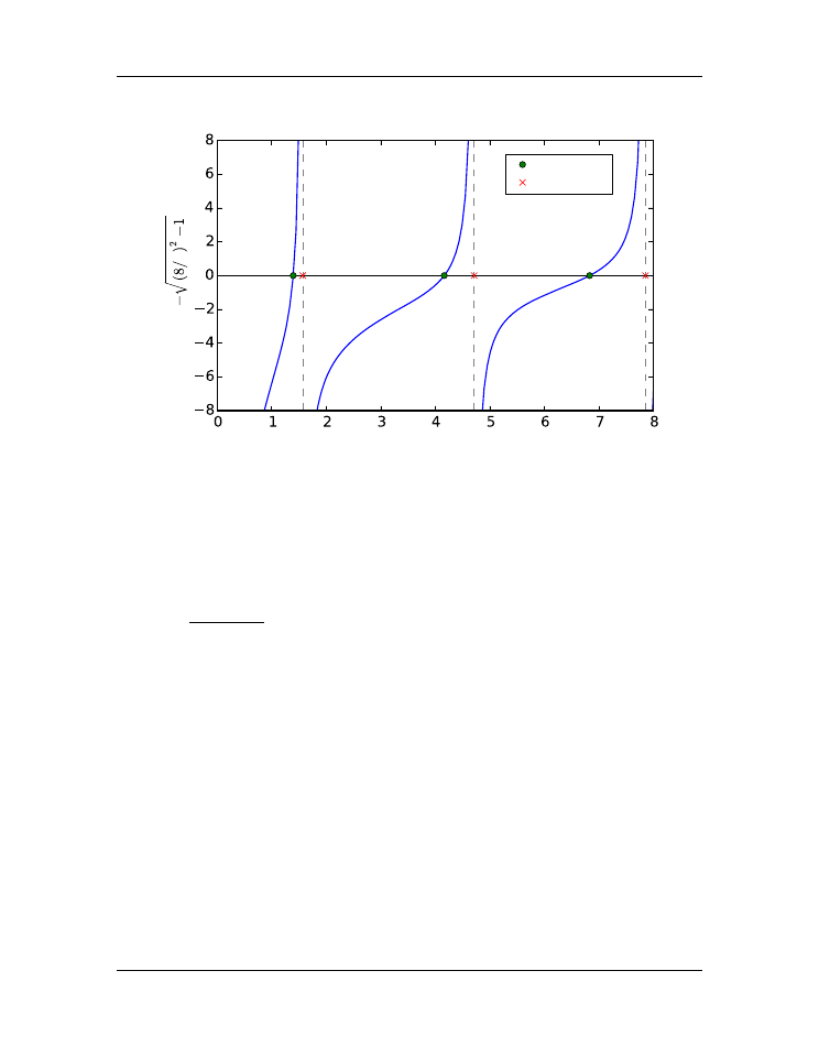
argument of the square root becomes negative. The solutions, the points where
f
(
x
) = 0
are indicated by green circles; there are three of them. Another notable feature of the
function is that it diverges to
±∞
at
x
=
{
0
, π/
2
,
3
π/
2
,
5
π/
2
}
.
Brent method
One of the workhorses for finding solutions to a single variable nonlinear equation is the
method of Brent, discussed in many texts on numerical methods. SciPy’s implementa-
tion of the Brent algorithm is the function
scipy.optimize.brentq(f, a, b)
,
which has three required arguments. The first
f
is the name of the user-defined function
166
Chapter 9. Numerical Routines: SciPy and NumPy

Introduction to Python for Science, Release 0.9.23
x
tan
x
x
true roots
false roots
Figure 9.2: Roots of a nonlinear function
to be solved. The next two,
a
and
b
are the
x
values that bracket the solution you are
looking for. You should choose
a
and
b
so that there is only one solutions in the inter-
val between
a
and
b
. Brent’s method also requires that
f(a)
and
f(b)
have opposite
signs; an error message is returned if they do not. Thus to find the three solutions to
tan
x
−
p
(8
/x
)
2
−
1 = 0
, we need to run
scipy.optimize.brentq(f, a, b)
three times using three different values of
a
and
b
that bracket each of the three solutions.
The program below illustrates the how to use
scipy.optimize.brentq
import
numpy
as
np
import
scipy
as
sp
import
matplotlib.pyplot
as
plt
def
tdl
(x):
y
=
8.
/
x
return
np
.
tan(x)
-
np
.
sqrt(y
*
y
-
1.0
)
# Find true roots
rx1
=
sp
.
optimize
.
brentq(tdl,
0.5
,
0.49
*
np
.
pi)
rx2
=
sp
.
optimize
.
brentq(tdl,
0.51
*
np
.
pi,
1.49
*
np
.
pi)
rx3
=
sp
.
optimize
.
brentq(tdl,
1.51
*
np
.
pi,
2.49
*
np
.
pi)
9.3. Solving non-linear equations
167

Introduction to Python for Science, Release 0.9.23
rx
=
np
.
array([rx1, rx2, rx3])
ry
=
np
.
zeros(
3
)
# print using a list comprehension
(
’
\n
True roots:’
)
(
’
\n
’
.
join(
’f({0:0.5f}) = {1:0.2e}’
.
format(x, tdl(x))
for
x
in
rx))
# Find false roots
rx1f
=
sp
.
optimize
.
brentq(tdl,
0.49
*
np
.
pi,
0.51
*
np
.
pi)
rx2f
=
sp
.
optimize
.
brentq(tdl,
1.49
*
np
.
pi,
1.51
*
np
.
pi)
rx3f
=
sp
.
optimize
.
brentq(tdl,
2.49
*
np
.
pi,
2.51
*
np
.
pi)
rxf
=
np
.
array([rx1f, rx2f, rx3f])
# print using a list comprehension
(
’
\n
False roots:’
)
(
’
\n
’
.
join(
’f({0:0.5f}) = {1:0.2e}’
.
format(x, tdl(x))
for
x
in
rxf))
# Plot function and various roots
x
=
np
.
linspace(
0.7
,
8
,
128
)
y
=
tdl(x)
# Create masked array for plotting
ymask
=
np
.
ma
.
masked_where(np
.
abs(y)
>
20.
, y)
plt
.
figure(figsize
=
(
6
,
4
))
plt
.
plot(x, ymask)
plt
.
axhline(color
=
’black’
)
plt
.
axvline(x
=
np
.
pi
/
2.
, color
=
"gray"
, linestyle
=
’--’
, zorder
=-
1
)
plt
.
axvline(x
=
3.
*
np
.
pi
/
2.
, color
=
"gray"
, linestyle
=
’--’
, zorder
=-
1
)
plt
.
axvline(x
=
5.
*
np
.
pi
/
2.
, color
=
"gray"
, linestyle
=
’--’
, zorder
=-
1
)
plt
.
xlabel(
r’$x$’
)
plt
.
ylabel(
r’$\tan x - \sqrt{(8/x)^2-1}$’
)
plt
.
ylim(
-
8
,
8
)
plt
.
plot(rx, ry,
’og’
, ms
=
5
, label
=
’true roots’
)
plt
.
plot(rxf, ry,
’xr’
, ms
=
5
, label
=
’false roots’
)
plt
.
legend(numpoints
=
1
, fontsize
=
’small’
, loc
=
’upper right’
,
bbox_to_anchor
=
(
0.92
,
0.97
))
plt
.
tight_layout()
plt
.
show()
Running this code generates the following output:
In [1]:
run rootbrentq
.
py
168
Chapter 9. Numerical Routines: SciPy and NumPy

Introduction to Python for Science, Release 0.9.23
True roots:
f(1.39547) = -6.39e-14
f(4.16483) = -7.95e-14
f(6.83067) = -1.11e-15
False roots:
f(1.57080) = -1.61e+12
f(4.71239) = -1.56e+12
f(7.85398) = 1.16e+12
The Brent method finds the three true roots of the equation quickly and accurately when
you provide values for the brackets
a
and
b
that are valid. However, like many numerical
methods for finding roots, the Brent method can produce spurious roots as it does in the
above example when
a
and
b
bracket singularities like those at
x
=
{
π/
2
,
3
π/
2
,
5
π/
2
}
.
Here we evaluated the function at the purported roots found by
brentq
to verify that
the values of
x
found were indeed roots. For the true roots, the values of the function
were very near zero, to within an acceptable roundoff error of less than
10
−
13
. For the
false roots, exceedingly large numbers on the order of
10
12
were obtained, indicating a
possible problem with these roots. These results, together with the plots, allow you to
unambiguously identify the true solutions to this nonlinear function.
The
brentq
function has a number of optional keyword arguments that you may find
useful. One keyword argument causes
brentq
to return not only the solution but the
value of the function evaluated at the solution. Other arguments allow you to specify a
tolerance to which the solution is found as well as a few other parameters possibly of
interest. Most of the time, you can leave the keyword arguments at their default values.
See the
brentq
entry online on the SciPy web site for more information.
Other methods for solving equations of a single variable
SciPy provides a number of other methods for solving nonlinear equations of a
single variable.
It has an implementation of the Newton-Raphson method called
scipy.optimize.newton
. It’s the racecar of such methods; its super fast but less
stable that the Brent method. To fully realize its speed, you need to specify not only the
function to be solved, but also its first derivative, which is often more trouble than its
worth. You can also specify its second derivative, which may further speed up finding the
solution. If you do not specify the first or second derivatives, the method uses the secant
method, which is usually slower than the Brent method.
Other methods, including the Ridder (
scipy.optimize.ridder
) and bisection
(
scipy.optimize.bisect
), are also available, although the Brent method is gen-
erally superior. SciPy let’s you use your favorite.
9.3. Solving non-linear equations
169