ВУЗ: Не указан
Категория: Не указан
Дисциплина: Не указана
Добавлен: 17.04.2021
Просмотров: 3742
Скачиваний: 3

Introduction to Python for Science, Release 0.9.23
9.3.2 Solving systems of nonlinear equations
Solving systems of nonlinear equations is not for the faint of heart. It is a difficult problem
that lacks any general purpose solutions. Nevertheless, SciPy provides quite an assort-
ment of numerical solvers for nonlinear systems of equations. However, because of the
complexity and subtleties of this class of problems, we do not discuss their use here.
9.4 Solving ODEs
The
scipy.integrate
library has two powerful powerful routines,
ode
and
odeint
, for numerically solving systems of coupled first order ordinary differential
equations (ODEs). While
ode
is more versatile,
odeint
(ODE integrator) has a simpler
Python interface works very well for most problems. It can handle both stiff and non-stiff
problems. Here we provide an introduction to
odeint
.
A typical problem is to solve a second or higher order ODE for a given set of initial
conditions. Here we illustrate using
odeint
to solve the equation for a driven damped
pendulum. The equation of motion for the angle
θ
that the pendulum makes with the
vertical is given by
d
2
θ
dt
2
=
−
1
Q
dθ
dt
+ sin
θ
+
d
cos Ω
t
where
t
is time,
Q
is the quality factor,
d
is the forcing amplitude, and
Ω
is the driving
frequency of the forcing. Reduced variables have been used such that the natural (angular)
frequency of oscillation is 1. The ODE is nonlinear owing to the
sin
θ
term. Of course,
it’s precisely because there are no general methods for solving nonlinear ODEs that one
employs numerical techniques, so it seems appropriate that we illustrate the method with
a nonlinear ODE.
The first step is always to transform any
n
th
-order ODE into a system of
n
first order
ODEs of the form:
dy
1
dt
=
f
1
(
t, y
1
, ..., y
n
)
dy
2
dt
=
f
2
(
t, y
1
, ..., y
n
)
..
.
=
..
.
dy
n
dt
=
f
n
(
t, y
1
, ..., y
n
)
.
170
Chapter 9. Numerical Routines: SciPy and NumPy

Introduction to Python for Science, Release 0.9.23
We also need
n
initial conditions, one for each variable
y
i
. Here we have a second order
ODE so we will have two coupled ODEs and two initial conditions.
We start by transforming our second order ODE into two coupled first order ODEs. The
transformation is easily accomplished by defining a new variable
ω
≡
dθ/dt
. With this
definition, we can rewrite our second order ODE as two coupled first order ODEs:
dθ
dt
=
ω
dω
dt
=
−
1
Q
ω
+ sin
θ
+
d
cos Ω
t .
In this case the functions on the right hand side of the equations are
f
1
(
t, θ, ω
) =
ω
f
2
(
t, θ, ω
) =
−
1
Q
ω
+ sin
θ
+
d
cos Ω
t .
Note that there are no explicit derivatives on the right hand side of the functions
f
i
; they
are all functions of
t
and the various
y
i
, in this case
θ
and
ω
.
The initial conditions specify the values of
θ
and
ω
at
t
= 0
.
SciPy’s ODE solver
scipy.integrate.odeint
has three required arguments and
many optional keyword arguments, of which we only need one,
args
, for this example.
So in this case,
odeint
has the form
odeint(func, y0, t, args=())
The first argument
func
is the name of a Python function that returns a list of values of
the
n
functions
f
i
(
t, y
1
, ..., y
n
)
at a given time
t
. The second argument
y0
is an array (or
list) of the values of the initial conditions of
y
1
, ..., y
n
)
. The third argument is the array
of times at which you want
odeint
to return the values of
y
1
, ..., y
n
)
. The keyword
argument
args
is a tuple that is used to pass parameters (besides
y0
and
t
) that are
needed to evaluate
func
. Our example should make all of this clear.
After having written the
n
th
-order ODE as a system of
n
first-order ODEs, the next task
is to write the function
func
. The function
func
should have three arguments: (1) the
list (or array) of current
y
values, the current time
t
, and a list of any other parameters
params
needed to evaluate
func
. The function
func
returns the values of the deriva-
tives
dy
i
/dt
=
f
i
(
t, y
1
, ..., y
n
)
in a list (or array). Lines 5-11 illustrate how to write
func
for our example of a driven damped pendulum. Here we name the function simply
f
, which is the name that appears in the call to
odeint
in line 33 below.
The only other tasks remaining are to define the parameters needed in the function,
bundling them into a list (see line 22 below), and to define the initial conditions, and
9.4. Solving ODEs
171

Introduction to Python for Science, Release 0.9.23
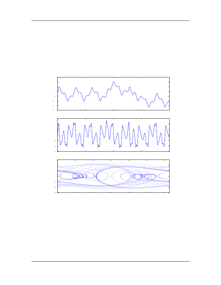
bundling them into another list (see line 25 below). After defining the time array in lines
28-30, the only remaining task is to call
odeint
with the appropriate arguments and a
variable,
psoln
in this case‘‘ to store output. The output
psoln
is an
n
element array
where each element is itself an array corresponding the the values of
y
i
for each time in
the time
t
array that was an argument of
odeint
. For this example, the first element
psoln[:,0]
is the
y
0
or
theta
array, and the second element
psoln[:,1]
is the
y
1
or
omega
array. The remainder of the code simply plots out the results in different
formats. The resulting plots are shown in the figure
after the code.
1
import
numpy
as
np
2
import
matplotlib.pyplot
as
plt
3
from
scipy.integrate
import
odeint
4
5
def
f
(y, t, params):
6
theta, omega
=
y
# unpack current values of y
7
Q, d, Omega
=
params
# unpack parameters
8
derivs
=
[omega,
# list of dy/dt=f functions
9
-
omega
/
Q
+
np
.
sin(theta)
+
d
*
np
.
cos(Omega
*
t)]
10
return
derivs
11
12
# Parameters
13
Q
=
2.0
# quality factor (inverse damping)
14
d
=
1.5
# forcing amplitude
15
Omega
=
0.65
# drive frequency
16
17
# Initial values
18
theta0
=
0.0
# initial angular displacement
19
omega0
=
0.0
# initial angular velocity
20
21
# Bundle parameters for ODE solver
22
params
=
[Q, d, Omega]
23
24
# Bundle initial conditions for ODE solver
25
y0
=
[theta0, omega0]
26
27
# Make time array for solution
28
tStop
=
200.
29
tInc
=
0.05
30
t
=
np
.
arange(
0.
, tStop, tInc)
31
32
# Call the ODE solver
33
psoln
=
odeint(f, y0, t, args
=
(params,))
34
35
# Plot results
36
fig
=
plt
.
figure(
1
, figsize
=
(
8
,
8
))
172
Chapter 9. Numerical Routines: SciPy and NumPy

Introduction to Python for Science, Release 0.9.23
37
38
# Plot theta as a function of time
39
ax1
=
fig
.
add_subplot(
311
)
40
ax1
.
plot(t, psoln[:,
0
])
41
ax1
.
set_xlabel(
’time’
)
42
ax1
.
set_ylabel(
’theta’
)
43
44
# Plot omega as a function of time
45
ax2
=
fig
.
add_subplot(
312
)
46
ax2
.
plot(t, psoln[:,
1
])
47
ax2
.
set_xlabel(
’time’
)
48
ax2
.
set_ylabel(
’omega’
)
49
50
# Plot omega vs theta
51
ax3
=
fig
.
add_subplot(
313
)
52
twopi
=
2.0
*
np
.
pi
53
ax3
.
plot(psoln[:,
0
]
%
twopi, psoln[:,
1
],
’.’
, ms
=
1
)
54
ax3
.
set_xlabel(
’theta’
)
55
ax3
.
set_ylabel(
’omega’
)
56
ax3
.
set_xlim(
0.
, twopi)
57
58
plt
.
tight_layout()
59
plt
.
show()
The plots above reveal that for the particular set of input parameters chosen
Q = 2.0
,
d = 1.5
, and
Omega = 0.65
, the pendulum trajectories are chaotic. Weaker forcing
(smaller
d
) leads to what is perhaps the more familiar behavior of sinusoidal oscillations
with a fixed frequency which, at long times, is equal to the driving frequency.
9.5 Discrete (fast) Fourier transforms
The SciPy library has a number of routines for performing discrete Fourier transforms.
Before delving into them, we provide a brief review of Fourier transforms and discrete
Fourier transforms.
9.5.1 Continuous and discrete Fourier transforms
The Fourier transform of a function
g
(
t
)
is given by
G
(
f
) =
Z
∞
−∞
g
(
t
)
e
−
i
2
πf t
dt ,
(9.1)
9.5. Discrete (fast) Fourier transforms
173
Introduction to Python for Science, Release 0.9.23
0
50
100
150
200
time
20
15
10
5
0
5
10
15
theta
0
50
100
150
200
time
3
2
1
0
1
2
3
omega
0
1
2
3
4
5
6
theta
3
2
1
0
1
2
3
omega
Figure 9.3: Pendulum trajectory
174
Chapter 9. Numerical Routines: SciPy and NumPy