ВУЗ: Не указан
Категория: Не указан
Дисциплина: Не указана
Добавлен: 17.04.2021
Просмотров: 3728
Скачиваний: 3

Introduction to Python for Science, Release 0.9.23
where
f
is the Fourier transform variable; if
t
is time, then
f
is frequency. The inverse
transform is given by
g
(
t
) =
Z
∞
−∞
G
(
f
)
e
i
2
πf t
df
(9.2)
Here we define the Fourier transform in terms of the frequency
f
rather than the angular
frequency
ω
= 2
πf
.
The conventional Fourier transform is defined for continuous functions, or at least for
functions that are dense and thus have an infinite number of data points. When doing
numerical analysis, however, you work with
discrete
data sets, that is, data sets defined for
a finite number of points. The discrete Fourier transform (DFT) is defined for a function
g
n
consisting of a set of
N
discrete data points. Those
N
data points must be defined at
equally-spaced
times
t
n
=
n
∆
t
where
∆
t
is the time between successive data points and
n
runs from 0 to
N
−
1
. The discrete Fourier transform (DFT) of
g
n
is defined as
G
l
=
N
−
1
X
n
=0
g
n
e
−
i
(2
π/N
)
ln
(9.3)
where
l
runs from 0 to
N
−
1
. The inverse discrete Fourier transform (iDFT) is defined
as
g
n
=
1
N
N
−
1
X
l
=0
G
l
e
i
(2
π/N
)
ln
.
(9.4)
The DFT is usually implemented on computers using the well-known Fast Fourier Trans-
form (FFT) algorithm, generally credited to Cooley and Tukey who developed it at AT&T
Bell Laboratories during the 1960s. But their algorithm is essentially one of many in-
dependent rediscoveries of the basic algorithm dating back to Gauss who described it as
early as 1805.
9.5.2 The SciPy FFT library
The SciPy library
scipy.fftpack
has routines that implement a souped-up version of
the FFT algorithm along with many ancillary routines that support working with DFTs.
The basic FFT routine in
scipy.fftpack
is appropriately named
fft
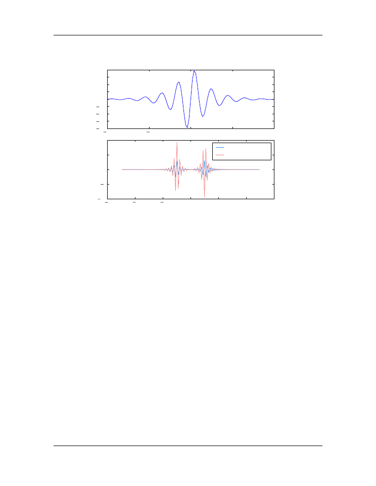
. The program
below illustrates its use, along with the plots that follow.
import
numpy
as
np
from
scipy
import
fftpack
import
matplotlib.pyplot
as
plt
9.5. Discrete (fast) Fourier transforms
175

Introduction to Python for Science, Release 0.9.23
width
=
2.0
freq
=
0.5
t
=
np
.
linspace(
-
10
,
10
,
101
)
# linearly space time array
g
=
np
.
exp(
-
np
.
abs(t)
/
width)
*
np
.
sin(
2.0
*
np
.
pi
*
freq
*
t)
dt
=
t[
1
]
-
t[
0
]
# increment between times in time array
G
=
fftpack
.
fft(g)
# FFT of g
f
=
fftpack
.
fftfreq(g
.
size, d
=
dt)
# frequenies f[i] of g[i]
f
=
fftpack
.
fftshift(f)
# shift frequencies from min to max
G
=
fftpack
.
fftshift(G)
# shift G order to coorespond to f
fig
=
plt
.
figure(
1
, figsize
=
(
8
,
6
), frameon
=
False
)
ax1
=
fig
.
add_subplot(
211
)
ax1
.
plot(t, g)
ax1
.
set_xlabel(
’t’
)
ax1
.
set_ylabel(
’g(t)’
)
ax2
=
fig
.
add_subplot(
212
)
ax2
.
plot(f, np
.
real(G), color
=
’dodgerblue’
, label
=
’real part’
)
ax2
.
plot(f, np
.
imag(G), color
=
’coral’
, label
=
’imaginary part’
)
ax2
.
legend()
ax2
.
set_xlabel(
’f’
)
ax2
.
set_ylabel(
’G(f)’
)
plt
.
show()
The DFT has real and imaginary parts, both of which are plotted in the figure.
The
fft
function returns the
N
Fourier components of
G
n
starting with the zero-
frequency component
G
0
and progressing to the maximum positive frequency compo-
nent
G
(
N/
2)
−
1
(or
G
(
N
−
1)
/
2
if
N
is odd). From there,
fft
returns the maximum
neg-
ative
component
G
N/
2
(or
G
(
N
−
1)
/
2
if
N
is odd) and continues upward in frequency
until it reaches the minimum negative frequency component
G
N
−
1
. This is the standard
way that DFTs are ordered by most numerical DFT packages. The
scipy.fftpack
function
fftfreq
creates the array of frequencies in this non-intuitive order such that
f[n]
in the above routine is the correct frequency for the Fourier component
G[n]
. The
arguments of
fftfreq
are the size of the the orignal array
g
and the keyword argu-
ment
d
that is the spacing between the (equally spaced) elements of the time array (
d=1
if left unspecified). The package
scipy.fftpack
provides the convenience function
fftshift
that reorders the frequency array so that the zero-frequency occurs at the
middle of the array, that is, so the frequencies proceed monotonically from smallest (most
176
Chapter 9. Numerical Routines: SciPy and NumPy
Introduction to Python for Science, Release 0.9.23
10
5
0
5
10
t
0.8
0.6
0.4
0.2
0.0
0.2
0.4
0.6
0.8
g(t)
3
2
1
0
1
2
3
f
10
5
0
5
10
G(f)
real part
imaginary part
Figure 9.4: Function
g
(
t
)
and its DFT
G
(
f
)
.
negative) to largest (most positive). Applying
fftshift
to both
f
and
G
puts the fre-
quencies
f
in ascending order and shifts
G
so that the frequency of
G[n]
is given by the
shifted
f[n]
.
The
scipy.fftpack
module also contains routines for performing 2-dimensional and
n
-dimensional DFTs, named
fft2
and
fftn
, respectively, using the FFT algorithm.
As for most FFT routines, the
scipy.fftpack
FFT routines are most efficient if
N
is
a power of 2. Nevertheless, the FFT routines are able to handle data sets where
N
is not
a power of 2.
scipy.fftpack
also supplies an inverse DFT function
ifft
. It is written to act on
the
unshifted
FFT so take care! Note also that
ifft
returns a
complex
array. Because
of machine roundoff error, the imaginary part of the function returned by
ifft
will, in
general, be very near zero but not exactly zero even when the original function is a purely
real function.
9.5. Discrete (fast) Fourier transforms
177

Introduction to Python for Science, Release 0.9.23
9.6 Exercises
1. Use NumPy’s
polyval
function together with SciPy to plot the following func-
tions:
(a) The first four Chebyshev polynomials of first kind. Plot these over the interval
from -1 to +1.
(b) The first four Hermite polynomials
multiplied
by
e
−
x
2
/
2
. Plot these on the
interval from -5 to +5. These are the first four wave functions of the quantum
mechanical simple harmonic oscillator.
178
Chapter 9. Numerical Routines: SciPy and NumPy

APPENDIX
A
INSTALLING PYTHON
For scientific programming with Python, you need to install Python and three scientific
Python libraries: NumPy, SciPy, and MatPlotLib. There are many more libraries you can
install, but Python along with NumPy, SciPy, and MatPlotLib are those that are essential
for scientific programming.
A.1 Installing Python
There are a number of ways to install Python and the scientific libraries you will need
on your computer. Some are easier than others. You can install Python and the scientific
libraries you need from “source” and compile them yourself. This is not recommended
unless you are an expert in Python, in which case you have little need for this manual.
For most people, the simplest way to install Python and all the scientific libraries you
need is to install either
Canopy
or
Spyder
. Canopy and Spyder are integrated development
environments (IDEs) for Python. They have a number of very useful features and tools.
First, they have syntax highlighting, which colors different parts Python syntax according
to function, making code easier to read. Second, and more importantly, they run a program
in the background called
PyFlakes
that checks the validity of the Python syntax as you
write it. It’s like a spelling and grammar checker all rolled into one, and it is extremely
useful, for novice and expert alike. The Canopy and Spyder IDEs have a number of other
useful features, which we do not go into here, but expect you will learn about as you
become more familiar with Python. Canopy is a simpler IDE than Spyder, and easier for
novices to learn and maintain. Spyder has more advanced features, which you may find
useful as you become more expert in Python programming.
Canopy
is written, maintained, and distributed by the software company Enthought
). There are two versions of Canopy. One version,
Canopy
179