ВУЗ: Не указан
Категория: Не указан
Дисциплина: Не указана
Добавлен: 17.04.2021
Просмотров: 3737
Скачиваний: 3

Introduction to Python for Science, Release 0.9.23
etc.
The call
ax2.set_yscale(’log’)
sets the
y
-axes in the second plot to be logarith-
mic, thus creating a semi-log plot. Creating properly-labeled logarthmic axes like this is
more straightforward with the advanced syntax illustrated in the above example.
Using the prefixes
ax1
,
ax2
, or
ax3
, direct graphical instructions to their respective
subplots. By creating and specifying names for the different figure windows and subplots
within them, you access the different plot windows more efficiently. For example, the
following code makes four identical subplots in a single figure window using a
for
loop.
In [1]:
fig
=
figure()
In [2]:
ax1
=
fig
.
add_subplot(
221
)
In [3]:
ax2
=
fig
.
add_subplot(
222
)
In [4]:
ax3
=
fig
.
add_subplot(
223
)
In [5]:
ax4
=
fig
.
add_subplot(
224
)
In [6]:
for
ax
in
[ax1, ax2, ax3, ax4]:
...:
ax
.
plot([
3
,
5
,
8
],[
6
,
3
,
1
])
In [7]:
show()
5.4. More advanced graphical output
95

Introduction to Python for Science, Release 0.9.23
5.5 Exercises
1. Plot the function
y
= 3
x
2
for
−
1
≤
x
≤
3
as a continuous line. Include enough
points so that the curve you plot appears smooth. Label the axes
x
and
y
.
2. Plot the following function for
−
15
≤
x
≤
15
:
y
=
cos
x
1 +
1
5
x
2
Include enough points so that the curve you plot appears smooth. Label the axes
x
and
y
.
3. Plot the functions
sin
x
and
cos
x
vs
x
on the same plot with
x
going from
−
π
to
π
. Make sure the limits of
x
-axis do not extend beyond the limits of the data. Plot
sin
x
in the color green and
cos
x
in the color black and include a legend to label the
two curves. Place the legend within the plot, but such that it does not cover either
of the sine or cosine traces.
4. Create a data file with the data shown below.
(a) Read the data into Python program and plot
t
vs
y
using circles for data points
with error bars. Use the data in the
dy
column as the error estimates for the
y
data. Label the horizontal and vertical axes “time (s)” and “position (cm)”.
(b) On the same graph, plot the function below as a smooth line. Make the line
pass
behind
the data points.
y
(
t
) =
3 +
1
2
sin
πt
5
t e
−
t/
10
Data for Exercise 4
Date: 16-Aug-2013
Data taken by Lauren and John
t
d
dy
1.0
2.94
0.7
4.5
8.29
1.2
8.0
9.36
1.2
11.5
11.60
1.4
15.0
9.32
1.3
18.5
7.75
1.1
22.0
8.06
1.2
25.5
5.60
1.0
96
Chapter 5. Plotting

Introduction to Python for Science, Release 0.9.23
29.0
4.50
0.8
32.5
4.01
0.8
36.0
2.62
0.7
39.5
1.70
0.6
43.0
2.03
0.6
5. Use MatPlotLib’s function
hist
along with NumPy’s function’s
random.rand
and
random.randn
to create the histogram graphs shown in Fig.
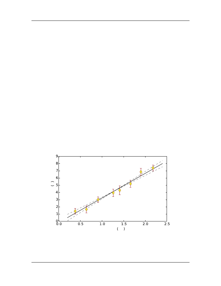
6. Plot force
vs
distance with error bars using the following data:
d
=
np
.
array([
0.38
,
0.64
,
0.91
,
1.26
,
1.41
,
1.66
,
1.90
,
2.18
])
f
=
np
.
array([
1.4
,
1.65
,
3.0
,
3.95
,
4.3
,
5.20
,
6.85
,
7.4
])
df
=
np
.
array([
0.4
,
0.5
,
0.4
,
0.5
,
0.6
,
0.5
,
0.5
,
0.4
])
Your plot should also include a visual straight “best fit” to the data as well as visual
“fits” that give the smallest and largest slopes consistent with the data. Note, you
only need two points to define a straight line so the straight lines you draw on the
plot should be arrays of length 2 and no longer. All of your fitted lines should lie
behind
the data. Try to make your plot look like the one below.
In addition
, add
a legend to your plot the gives the slope with its uncertainty obtained from your
visual fits to the data.
distance cm
for
ce
N
The web page
http://matplotlib.org/api/pyplot_summary.html
gives a summary of
the main plotting commands available in MatPlotLib. The two important ones here
5.5. Exercises
97

Introduction to Python for Science, Release 0.9.23
are
plot
and
errorbar
, which make regular plots and plots with error bars,
respectively. You will find the following keyword arguments useful:
yerr
,
ls
,
marker
,
mfc
,
mec
,
ms
, and
ecolor
, which you can find described by clicking
on the
errorbar
function link on the web page cited above.
7. The data file below shows data obtained for the displacement (position)
vs
time of
a falling object, together with the estimated uncertainty in the displacement.
Measurements of fall velocity vs time
Taken by A.P. Crawford and S.M. Torres
19-Sep-13
time (s)
position (m)
uncertainty (m)
0.0
0.0
0.04
0.5
1.3
0.12
1.0
5.1
0.2
1.5
10.9
0.3
2.0
18.9
0.4
2.5
28.7
0.4
3.0
40.3
0.5
3.5
53.1
0.6
4.0
67.5
0.6
4.5
82.3
0.6
5.0
97.6
0.7
5.5
113.8
0.7
6.0
131.2
0.7
6.5
148.5
0.7
7.0
166.2
0.7
7.5
184.2
0.7
8.0
201.6
0.7
8.5
220.1
0.7
9.0
238.3
0.7
9.5
256.5
0.7
10.0
275.6
0.8
(a) Use these data to calculate the velocity and acceleration (in a Python program
.py
file), together with their uncertainties propagated from the displacement
vs
time uncertainties. Be sure to calculate time arrays corresponding the mid-
point in time between the two displacements or velocities for the velocity and
acceleration arrays, respectively.
(b) In a single window frame, make three vertically stacked plots of the displace-
ment, velocity, and acceleration
vs
time. Show the error bars on the different
plots. Make sure that the time axes of all three plots cover the same range of
times. Why do the relative sizes of the error bars grow progressively greater
as one progresses from displacement to velocity to acceleration?
98
Chapter 5. Plotting

CHAPTER
SIX
CONDITIONALS AND LOOPS
Computer programs are useful for performing repetitive tasks. Without complaining, get-
ting bored, or growing tired, they can repetitively perform the same calculations with
minor, but important, variations over and over again. Humans share with computers none
of these qualities. And so we humans employ computers to perform the massive repetitive
tasks we would rather avoid. However, we need efficient ways of telling the computer to
do these repetitive tasks; we don’t want to have stop to tell the computer each time it
finishes one iteration of a task to do the task again, but for a slightly different case. We
want to tell it once, “Do this task 1000 times with slightly different conditions and report
back to me when you are done.” This is what
loops
were made for.
In the course of doing these repetitive tasks, computers often need to make decisions. In
general, we don’t want the computer to stop and ask us what it should do if a certain result
is obtained from its calculations. We might prefer to say, “Look, if you get result A during
your calculations, do this, otherwise, do this other thing.” That is, we often want to tell
the computer ahead of time what to do if it encounters different situations. This is what
conditionals
were made for.
Conditionals and loops control the flow of a program. They are essential to perform-
ing virtually any significant computational task. Python, like most computer languages,
provides a variety of ways of implementing loops and conditionals.
6.1 Conditionals
Conditional statements allow a computer program to take different actions based on
whether some condition, or set of conditions is true or false. In this way, the programmer
can control the flow of a program.
99